Understanding Aggregate Demand and Monetary Markets
Explore the interplay between planned investment, interest rates, and equilibrium in goods and money markets using the IS-LM model. Learn about policy effects, the macroeconomic policy mix, and shifts in the aggregate demand curve.

Understanding Aggregate Demand and Monetary Markets
E N D
Presentation Transcript
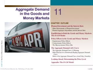
Aggregate Demand in the Goods and Money Markets 11 CHAPTER OUTLINE Planned Investment and the Interest Rate Other Determinants of Planned Investment Planned Aggregate Expenditure and the Interest Rate Equilibrium in Both the Goods and Money Markets: The IS-LM Model Policy Effects in the Goods and Money Markets Expansionary Policy Effects Contractionary Policy Effects The Macroeconomic Policy Mix The Aggregate Demand (AD) Curve The Aggregate Demand Curve: A Warning Other Reasons for a Downward-Sloping Aggregate Demand Curve Shifts of the Aggregate Demand Curve from Policy Variables Looking Ahead: Determining the Price Level Appendix: The IS-LM Model
goods marketThe market in which goods and services are exchanged and in which the equilibrium level of aggregate output is determined. money marketThe market in which financial instruments are exchanged and in which the equilibrium level of the interest rate is determined.
Planned Investment and the Interest Rate FIGURE 12.1 Planned Investment Schedule Planned investment spending is a negative function of the interest rate. An increase in the interest rate from 3 percent to 6 percent reduces planned investment from I0 to I1.
Reducing the interest rate, ceteris paribus, is likely to: a. Increase the level of planned investment spending. b. Decrease the level of planned investment. c. Shift the demand for money curve to the right. d. Shift the supply of money curve to the right.
Reducing the interest rate, ceteris paribus, is likely to: a. Increase the level of planned investment spending. b. Decrease the level of planned investment. c. Shift the demand for money curve to the right. d. Shift the supply of money curve to the right.
Planned Investment and the Interest Rate Other Determinants of Planned Investment The assumption that planned investment depends only on the interest rate is obviously a simplification, just as is the assumption that consumption depends only on income. In practice, the decision of a firm on how much to invest depends on, among other things, its expectation of future sales. The optimism or pessimism of entrepreneurs about the future course of the economy can have an important effect on current planned investment. Keynes used the phrase animal spirits to describe the feelings of entrepreneurs, and he argued that these feelings affect investment decisions.
Planned Investment and the Interest Rate Planned Aggregate Expenditure and the Interest Rate We can use the fact that planned investment depends on the interest rate to consider how planned aggregate expenditure (AE) depends on the interest rate. Recall that planned aggregate expenditure is the sum of consumption, planned investment, and government purchases. That is, AE ≡ C + I + G
Planned Investment and the Interest Rate Planned Aggregate Expenditure and the Interest Rate FIGURE 12.2 The Effect of an Interest Rate Increase on Planned Aggregate Expenditure An increase in the interest rate from 3 percent to 6 percent lowers planned aggregate expenditure and thus reduces equilibrium income from Y0 to Y1.
Planned Investment and the Interest Rate Planned Aggregate Expenditure and the Interest Rate • The effects of a change in the interest rate include: • A high interest rate (r) discourages planned investment (I). • Planned investment is a part of planned aggregate expenditure (AE). • Thus, when the interest rate rises, planned aggregate expenditure (AE) at every level of income falls. • Finally, a decrease in planned aggregate expenditure lowers equilibrium output (income) (Y) by a multiple of the initial decrease in planned investment.
Fill in the blanks. A higher interest rate __________ planned investment and causes planned aggregate expenditure to shift ___________. a. increases; upward b. increases; downward c. decreases; upward d. decreases; downward
Fill in the blanks. A higher interest rate __________ planned investment and causes planned aggregate expenditure to shift ___________. a. increases; upward b. increases; downward c. decreases; upward d. decreases; downward
Planned Investment and the Interest Rate Planned Aggregate Expenditure and the Interest Rate Using a convenient shorthand:
Equilibrium in Both the Goods and Money Markets: The IS-LM Model An increase in the interest rate (r) decreases output (Y) in the goods market because an increase in r lowers planned investment. When income (Y) increases, this shifts the money demand curve to the right, which increases the interest rate (r) with a fixed money supply. We can thus write:
Which of the following statements describes the relationship between the goods market and the money market? a. An increase in money demand. b. An increase in money supply. c. A decrease in the interest rate. d. An increase in both the supply and the demand for money.
Which of the following statements describes the relationship between the goods market and the money market? a. An increase in money demand. b. An increase in money supply. c. A decrease in the interest rate. d. An increase in both the supply and the demand for money.
Equilibrium in Both the Goods and Money Markets: The IS-LM Model FIGURE 12.3 Links between the Goods Market and the Money Market Planned investment depends on the interest rate, and money demand depends on aggregate output.
Which of the following is a link between the goods market and the money market? a. Income has considerable influence on the demand for money in the money market. b. The interest rate has significant effects on planned investment in the goods market. c. Both a and b above. d. None of the above. The goods market and the money market are not linked in the ways described above.
Which of the following is a link between the goods market and the money market? a. Income has considerable influence on the demand for money in the money market. b. The interest rate has significant effects on planned investment in the goods market. c. Both a and b above. d. None of the above. The goods market and the money market are not linked in the ways described above.
Policy Effects in the Goods and Money Markets Expansionary Policy Effects expansionary fiscal policyAn increase in government spending or a reduction in net taxes aimed at increasing aggregate output (income) (Y). expansionary monetary policyAn increase in the money supply aimed at increasing aggregate output (income) (Y).
Which of the following policy changes would be considered expansionary monetary policy? a. An increase in the money supply. b. An increase in net taxes. c. An increase in government spending. d. An increase in government borrowing.
Which of the following policy changes would be considered expansionary monetary policy? a. An increase in the money supply. b. An increase in net taxes. c. An increase in government spending. d. An increase in government borrowing.
Policy Effects in the Goods and Money Markets Expansionary Policy Effects Expansionary Fiscal Policy: An Increase in Government Purchases (G) or a Decrease in Net Taxes (T) crowding-out effectThe tendency for increases in government spending to cause reductions in private investment spending.
Policy Effects in the Goods and Money Markets Expansionary Policy Effects Expansionary Fiscal Policy: An Increase in Government Purchases (G) or a Decrease in Net Taxes (T) FIGURE 12.4 The Crowding-Out Effect An increase in government spending G from G0 to G1 shifts the planned aggregate expenditure schedule from 1 to 2. The crowding-out effect of the decrease in planned investment (brought about by the increased interest rate) then shifts the planned aggregate expenditure schedule from 2 to 3.
An increase in government spending (G), a. Increases planned aggregate expenditure, increases aggregate output, but may also cause a decrease in planned investment, which reduces both planned aggregate expenditure and aggregate output. b. Increases planned aggregate expenditure, increases aggregate output, and spurs even more planned investment, which further increases aggregate output. c. Decreases aggregate expenditure, planned investment, and aggregate output. d. All of the cases above have equal chance of occurring.
An increase in government spending (G), a. Increases planned aggregate expenditure, increases aggregate output, but may also cause a decrease in planned investment, which reduces both planned aggregate expenditure and aggregate output. b. Increases planned aggregate expenditure, increases aggregate output, and spurs even more planned investment, which further increases aggregate output. c. Decreases aggregate expenditure, planned investment, and aggregate output. d. All of the cases above have equal chance of occurring.
Effects of an expansionary fiscal policy: Policy Effects in the Goods and Money Markets Expansionary Policy Effects Expansionary Fiscal Policy: An Increase in Government Purchases (G) or a Decrease in Net Taxes (T) interest sensitivity or insensitivity of planned investmentThe responsiveness of planned investment spending to changes in the interest rate. Interest sensitivity means that planned investment spending changes a great deal in response to changes in the interest rate; interest insensitivity means little or no change in planned investment as a result of changes in the interest rate.
Effects of an expansionary monetary policy: Policy Effects in the Goods and Money Markets Expansionary Policy Effects Expansionary Monetary Policy: An Increase in the Money Supply
Effects of a contractionary fiscal policy: Policy Effects in the Goods and Money Markets Contractionary Policy Effects Contractionary Fiscal Policy: A Decrease in Government Spending (G) or an Increase in Net Taxes (T) contractionary fiscal policyA decrease in government spending or an increase in net taxes aimed at decreasing aggregate output (income) (Y).
Effects of a contractionary monetary policy: Policy Effects in the Goods and Money Markets Contractionary Policy Effects Contractionary Monetary Policy: A Decrease in the Money Supply contractionary monetary policyA decrease in the money supply aimed at decreasing aggregate output (income) (Y).
Policy Effects in the Goods and Money Markets The Macroeconomic Policy Mix policy mixThe combination of monetary and fiscal policies in use at a given time.
Which policy mix favors investment spending over government spending? a. Expansionary fiscal policy and contractionary monetary policy. b. An increase in the money supply and a fall in government purchases. c. Both expansionary fiscal policy and expansionary monetary policy. d. None of the above. No policy mix favors investment over government spending.
Which policy mix favors investment spending over government spending? a. Expansionary fiscal policy and contractionary monetary policy. b. An increase in the money supply and a fall in government purchases. c. Both expansionary fiscal policy and expansionary monetary policy. d. None of the above. No policy mix favors investment over government spending.
The Aggregate Demand (AD) Curve aggregate demand (AD) curveA curve that shows the negative relationship between aggregate output (income) and the price level. Each point on the AD curve is a point at which both the goods market and the money market are in equilibrium.
The Aggregate Demand (AD) Curve FIGURE 12.5 The Impact of an Increase in the Price Level on the Economy—Assuming No Changes in G, T, and Ms This figure shows that when P increases, Y decreases.
The Aggregate Demand (AD) Curve FIGURE 12.6 The Aggregate Demand (AD) Curve At all points along the AD curve, both the goods market and the money market are in equilibrium. The policy variables G, T, and Ms are fixed.
Let P equal the aggregate price level. Assuming that G, T, and MS remain the same, the impact of an increase in the price level on the economy can be described as follows: a. b. c. d. e.
Let P equal the aggregate price level. Assuming that G, T, and MS remain the same, the impact of an increase in the price level on the economy can be described as follows: a. b. c. d. e.
The Aggregate Demand (AD) Curve The Aggregate Demand Curve: A Warning It is important that you realize what the aggregate demand curve represents. The aggregate demand curve is more complex than a simple individual or market demand curve. The AD curve is not a market demand curve, and it is not the sum of all market demand curves in the economy. To understand what the aggregate demand curve represents, you must understand the interaction between the goods market and the money markets.
The Aggregate Demand (AD) Curve Other Reasons for a Downward-Sloping Aggregate Demand Curve The Consumption Link The consumption link provides another reason for the AD curve’s downward slope. An increase in the price level increases the demand for money, which leads to an increase in the interest rate, which leads to a decrease in consumption (as well as planned investment), which leads to a decrease in aggregate output (income). The initial decrease in consumption (brought about by the increase in the interest rate) contributes to the overall decrease in output.
The Aggregate Demand (AD) Curve Other Reasons for a Downward-Sloping Aggregate Demand Curve The Real Wealth Effect real wealth, or real balance, effectThe change in consumption brought about by a change in real wealth that results from a change in the price level.
The Aggregate Demand (AD) Curve Shifts of the Aggregate Demand Curve from Policy Variables FIGURE 12.7 The Effect of an Increase in Money Supply on the AD Curve An increase in the money supply (Ms) causes the aggregate demand curve to shift to the right, from AD0 to AD1. This shift occurs because the increase in Ms lowers the interest rate, which increases planned investment (and thus planned aggregate expenditure). The final result is an increase in output at each possible price level.
The Aggregate Demand (AD) Curve Shifts of the Aggregate Demand Curve from Policy Variables FIGURE 12.8 The Effect of an Increase in Government Purchases or a Decrease in Net Taxes on the AD Curve An increase in government purchases (G) or a decrease in net taxes (T) causes the aggregate demand curve to shift to the right, from AD0 to AD1. The increase in G increases planned aggregate expenditure, which leads to an increase in output at each possible price level. A decrease in T causes consumption to rise. The higher consumption then increases planned aggregate expenditure, which leads to an increase in output at each possible price level.
Along the aggregate demand curve, each point represents: a. Equilibrium in the goods market, regardless of the equilibrium situation in the money market. b. Equilibrium in the money market, regardless of the equilibrium situation in the goods market. c. Simultaneous equilibrium in both the goods and money markets. d. Macroeconomic equilibrium, or equilibrium in all markets of the economy.
Along the aggregate demand curve, each point represents: a. Equilibrium in the goods market, regardless of the equilibrium situation in the money market. b. Equilibrium in the money market, regardless of the equilibrium situation in the goods market. c. Simultaneous equilibrium in both the goods and money markets. d. Macroeconomic equilibrium, or equilibrium in all markets of the economy.
The Aggregate Demand (AD) Curve Shifts of the Aggregate Demand Curve from Policy Variables FIGURE 12.9 Factors That Shift the Aggregate Demand Curve
Which of the following policy mixes consistently shifts the aggregate demand curve to the right? a. Expansionary monetary policy accompanied by contractionary fiscal policy. b. Contractionary monetary policy accompanied by contractionary fiscal policy. c. Contractionary monetary policy accompanied by expansionary fiscal policy. d. Expansionary monetary policy accompanied by expansionary fiscal policy.
Which of the following policy mixes consistently shifts the aggregate demand curve to the right? a. Expansionary monetary policy accompanied by contractionary fiscal policy. b. Contractionary monetary policy accompanied by contractionary fiscal policy. c. Contractionary monetary policy accompanied by expansionary fiscal policy. d. Expansionary monetary policy accompanied by expansionary fiscal policy.
Looking Ahead: Determining the Price Level Our discussion of aggregate output (income) and the interest rate in the goods and money markets is now complete. You should have a good understanding of how the two markets work together. The AD curve is a useful summary of this analysis in that every point on the curve corresponds to equilibrium in both the goods and money markets for the given value of the price level. We have not yet, however, determined the price level. This is the task of the next chapter.
R E V I E W T E R M S A N D C O N C E P T S aggregate demand (AD) curve contractionary fiscal policy contractionary monetary policy crowding-out effect expansionary fiscal policy expansionary monetary policy goods market interest sensitivity or insensitivity of planned investment money market policy mix real wealth, or real balance, effect
CHAPTER 12 APPENDIX The IS-LM Model The IS Curve FIGURE 12A.1 The IS Curve Each point on the IS curve corresponds to the equilibrium point in the goods market for the given interest rate. When government spending (G) increases, the IS curve shifts to the right, from IS0 to IS1.