Random Number Generators
Random Number Generators. Why do we need random variables?. random components in simulation → need for a method which generates numbers that are random examples interarrival times service times demand sizes. terminology. Random Numbers

Random Number Generators
E N D
Presentation Transcript
Why do we need random variables? • random components in simulation → need for a method which generates numbers that are random • examples • interarrival times • service times • demand sizes 040669 || WS 2008 || Dr. Verena Schmid || PR KFK PM/SCM/TL Praktikum Simulation I
terminology • Random Numbers • stochastic variable that meets certain conditions • numbers randomly drawn from some known distribution • It is impossible to “generate” them with the help of a digital computer. • Pseudo-random Numbers • numbers which seem to be randomly drawn from some known distribution • may be generated with the help of a digital computer 040669 || WS 2008 || Dr. Verena Schmid || PR KFK PM/SCM/TL Praktikum Simulation I
techniques for generating random variables • ten-sided die (each throw generates a decimal) • throwing a coin n times • get a binary number between 0 and 2^n-1 • other physical devices • observe substances undergoing atomic decay • e.g., Caesium-137, Krypton-85,. . . 040669 || WS 2008 || Dr. Verena Schmid || PR KFK PM/SCM/TL Praktikum Simulation I
techniques for generating pseudo-random variables 1 0 1 0 1 • numbers are generated using a recursive formula • ri is a function of ri-1, ri-2, … • relation is deterministic – no random numbers • if the mathematical relation not known and well chosen it is practically impossible to predict the next number • In most cases we want the generated random numbers to simulate a uniform distribution over (0, 1), that is a U(0, 1)-distribution • there’re many simple techniques to transform uniform (U(a, b)) samples into samples from other well-known distributions 040669 || WS 2008 || Dr. Verena Schmid || PR KFK PM/SCM/TL Praktikum Simulation I
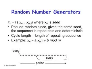
terminology • seed • random number generators are usually initialized with a starting number which is called the “seed” • different seeds generates different streams of pseudorandom numbers • the same seed results in the same stream • cycle length • length of the stream of pseudorandom numbers without repetition 040669 || WS 2008 || Dr. Verena Schmid || PR KFK PM/SCM/TL Praktikum Simulation I
methods for generating pseudo-random variables • all methods usually generate uniformly distributed pseudorandom numbers in the interval [0,1] • midsquare method (outdated) • congruential method (popular) • shift register (Tausworthe generator) 040669 || WS 2008 || Dr. Verena Schmid || PR KFK PM/SCM/TL Praktikum Simulation I
midsquare method • arithmetic generator • proposed by von Neumann and Metropolis in 1940s • algorithm • start with an initial number Z0 with m digits (seed) [m even] • square it and get a number with 2m digits (add a zero at the beginning if the number has only 2m-1 digits) • obtain Z1 by taking the middle m digits • to be in the interval [0,1) divide the Zi by 10m • etc…. 040669 || WS 2008 || Dr. Verena Schmid || PR KFK PM/SCM/TL Praktikum Simulation I
midsquare method: example (Z0 = 7182, m = 4) i 0 1 2 3 4 5 6 7 … Zi 7182 5811 7677 9363 6657 3156 9603 2176 … Ui 0.7182 0.5811 0.7677 0.9363 0.6657 0.3156 0.9603 0.2176 … Zi2 51581124 33767721 58936329 87665769 44315649 9960336 92217609 4734976 … 040669 || WS 2008 || Dr. Verena Schmid || PR KFK PM/SCM/TL Praktikum Simulation I
midsquare method (cont.) • advantages • fairly simple • disadvantage • tends to degenerate fairly rapidly to zero • example: try Z0 = 1009 • not random as predictable 040669 || WS 2008 || Dr. Verena Schmid || PR KFK PM/SCM/TL Praktikum Simulation I
Linear Congruential Generator (LCG) • LCGs • first proposed by Lehmer (1951). • produce pseudorandom numbers such that each single number determines its successor by means of a linear function followed by a modular reduction • to be in the interval [0,1) divide the Zi by m • Z0 seed a multiplier (integer) • c increment (integer) m modulus (integer) • Variations are possible • combinations of previous numbers instead of using only the last value 040669 || WS 2008 || Dr. Verena Schmid || PR KFK PM/SCM/TL Praktikum Simulation I
a = 5 c = 3 m = 16 Z0 = 7 LCG: example i 0 1 2 3 4 5 6 7 … Zi 7 6 1 8 11 10 5 12 … Ui 0.4375 0.375 0.0625 0.5 0.6875 0.625 0.3125 0.75 … Z1 = (5*Z0 + 3) mod 16 = 38 mod 16 = 6 Z2 = (5*Z1 + 3) mod 16 = 33 mod 16 = 1 Z3 = (5*Z2 + 3) mod 16 = 8 mod 16 = 8 … 040669 || WS 2008 || Dr. Verena Schmid || PR KFK PM/SCM/TL Praktikum Simulation I
properties of LCGs • parameters need to be chosen carefully • nonnegative • 0 < m a < m c < m Z0 < m • disadvantages • not random • if a and m are properly chosen, the Uis will “look like” they are randomly and uniformly distributed between 0 and 1. • can only take rational values 0, 1/m, 2/m, … (m-1)/m • looping 040669 || WS 2008 || Dr. Verena Schmid || PR KFK PM/SCM/TL Praktikum Simulation I
LCG (cont.) • looping • whenever Zi takes on a value it has had previously, exactly the same sequence of values is generated, and this cycle repeats itself endlessly. • length of sequence = period of generator • period can be at most m • if so: LCG has full period • LCG has full period iff • the only positive integer that divides both m and c is 1 • if q is a prime number that divides m then q divides a-1 • if 4 divides m, then 4 divides a-1 040669 || WS 2008 || Dr. Verena Schmid || PR KFK PM/SCM/TL Praktikum Simulation I
Linear Feedback Shift Register Generators (LFSR) • developed by Tausworthe (1965) • related to cryptographic methods • operate directly on bits to form random numbers • linear combination of the last q bits • ci constants (equal to 0 or 1, cq = 1) • in most applications only two of the cj coefficients are nonzero • execution can be spedup • modulo 2 equivalent to exclusive-or 040669 || WS 2008 || Dr. Verena Schmid || PR KFK PM/SCM/TL Praktikum Simulation I
LFSR (cont.) • form a sequence of binary integers W1, W2, … • string together l consecutive bits • consider them as numbers in base 2 • transform them into Uis • maximum period 2q -1 • if l is relatively prime to 2q-1 LFSR has full period 040669 || WS 2008 || Dr. Verena Schmid || PR KFK PM/SCM/TL Praktikum Simulation I
LFSR : example r = 3 q = 5 b1 = b2 = b3 = b4 = b5 = 1 l = 4 040669 || WS 2008 || Dr. Verena Schmid || PR KFK PM/SCM/TL Praktikum Simulation I
Testing RNGs Empirical Tests 040669 || WS 2008 || Dr. Verena Schmid || PR KFK PM/SCM/TL Praktikum Simulation I
random number generators • methods presented so far… • completely deterministic • Uisappear as if they were U(0,1) • test their actual quality • how well do the generated Uisresemble values of true IID U(0,1) • different kinds of tests • empirical tests • based on actual Uis produced by RNG • theoretical tests 040669 || WS 2008 || Dr. Verena Schmid || PR KFK PM/SCM/TL Praktikum Simulation I
Chi-Square test (with all parameters known) • checks whether the Uis appear to be IID U(0,1) • divide [0,1] into k subintervals of equal length (k > 100) • generate n random variables: U1, U2, .. Un • calculate fj(number of Uis that fall into jth subinterval) • calculate test statistic • for large n χ2 will have an approximate chi-square distribution with k-1 df under the null hypothesis that the Uis are IID U(0,1) • reject null hypothesis at level ® if 040669 || WS 2008 || Dr. Verena Schmid || PR KFK PM/SCM/TL Praktikum Simulation I
Generating Random Variates • General Approach • Inverse Transformation • Composition • Convolution • Generating Continuous Random Variates • Uniform U(a,b) • Exponential • m-Erlang • Gamma, Weibull • Normal • etc… 040669 || WS 2008 || Dr. Verena Schmid || PR KFK PM/SCM/TL Praktikum Simulation I
Inverse Transformation • generate continuous random variate X • distribution function F (continuous, strictly increasing) • 0 < F(x) < 1 • if x1 < x2 then 0 < F(x1) · F(x2) < 1 • inverse of F: F-1 • algorithm • generate U ~ U(0,1) • return X = F-1(U) 040669 || WS 2008 || Dr. Verena Schmid || PR KFK PM/SCM/TL Praktikum Simulation I
Inverse Transformation (cont.) F(x) 1 U1 U2 x 0 X2 X1 040669 || WS 2008 || Dr. Verena Schmid || PR KFK PM/SCM/TL Praktikum Simulation I returned value X has desired distribution F
Inverse Transformation (cont.) take natural logarithm (base e) create X according to exponential distribution with mean ¯ in order to find F-1 set 040669 || WS 2008 || Dr. Verena Schmid || PR KFK PM/SCM/TL Praktikum Simulation I
Inverse Transformation for discrete variates • distribution function • probability mass function • algorithm • generate U ~ U(0,1) • determine smallest possible integer i such that U ·F(xi) • return X = xi 040669 || WS 2008 || Dr. Verena Schmid || PR KFK PM/SCM/TL Praktikum Simulation I
Composition • applies then the distribution function F can be expressed as a convex combination of other distribution functions F1, F2, .. • we hope to be able to sample from the Fj’s more easily than from the original F • if X has a density it can be written as • algorithm • generate positive random integer J such that P(J = j) = pj • Return X with distribution function FJ 040669 || WS 2008 || Dr. Verena Schmid || PR KFK PM/SCM/TL Praktikum Simulation I
Composition (example) • double-exponential distribution (laplace distribution) • can be rewritten as • where IA(x) is the indicator function of set A • f(x) is a convex combination of • f1(x) = ex I(-1, 0) and f2(x) = e-x I[0,1) • p1 = p2 = 0.5 040669 || WS 2008 || Dr. Verena Schmid || PR KFK PM/SCM/TL Praktikum Simulation I
Convolution • desired random variable X can be expressed as sum of other random variables that are IID and can be generated more readily then X directly • algorithm • generate Y1, Y2, … Ym IID each with distribution function G • return X = Y1 + Y2 + + Ym • example: m-Erlang random variable X with mean ¯ • sum of m IID exponential random variables with common mean ¯/m 040669 || WS 2008 || Dr. Verena Schmid || PR KFK PM/SCM/TL Praktikum Simulation I
Generate Continuous Variates • Uniform distribution X(a,b) X = a + (b-a)U • Exponential (mean ¯) X = - ¯ln (1-U) or X = -¯ln U • m-Erlang 040669 || WS 2008 || Dr. Verena Schmid || PR KFK PM/SCM/TL Praktikum Simulation I