6.899 Relational Data Learning
6.899 Relational Data Learning. Yuan Qi MIT Media Lab yuanqi@media.mit.edu May 7, 2002. Outline. Structure Learning Using Stochastic Logic Programming (SLP) Text Classification Using Probabilistic Relational Models (PRM). Part 1:Structure Learning Using SLP.

6.899 Relational Data Learning
E N D
Presentation Transcript
6.899 Relational Data Learning Yuan Qi MIT Media Lab yuanqi@media.mit.edu May 7, 2002
Outline • Structure Learning Using Stochastic Logic Programming (SLP) • Text Classification Using Probabilistic Relational Models (PRM)
Part 1:Structure Learning Using SLP • SLP defines prior over BN structures • MCMC sampling BN structures • New Sampling Method
An SLP Defining prior BN structures bn([],[],[]). bn([RV|RVs],BN,AncBN):- bn(RVs, BN2, AncBN2), connect_no_cycles(RV,BN2,AncBN2,BN,AncBN). % An edge: RV parent of H 1/3:: which_edge([H|T],RV,[H-RV|Rest]):- choose_edges(T,RV,Rest). % An edge: H parent of RV 1/3:: which_edge([H|T],RV,[RV-H|Rest]) :- choose_edges(T,RV,Rest). % No edge 1/3:: which_edge([_H|T],RV,Rest) :- choose_edges(T,RV,Rest).
Metropolis-Hasting Sampling p(T) specifies a tree prior for BN structures. • Sampling T* from the transition distribution q(Ti,T*). • Set Ti = T* with the acceptance ratio else set Ti+1 = Ti.
The Transition Kernel (1) The transition kernel can be implemented by generating a new derivation(yielding a new model M*) from the derivation which yields the current model Mi. To be specific, we have • Backtrack one step to the most recent choice point in the SLD-tree (i.e., the probability tree) • If at the top of the tree, stop. Otherwise, backtrack one more step to the next choice point with a predefined backtrack probability pb.
The Transition Kernel (2) • Once stopped backtracking, choose a new leaf M* from the choice point by selecting branches according to their probabilities attached to them (loglinear sampling). However, we may not choose the branch that leads back to Mi.
Sampling Problems • Inefficiency of the previous Metropolis-Hasting sampling. pb =0.8, Acceptance ratio: 4%. • lf pb is small, slow movement of the samples, higher acceptance ratio • lf pb is large, large movement of the samples, lower acceptance ratio Fixed pb: the balance between local jumps to neighboring models and big jumps to distant ones. An Improvement: Cyclic transition kernel pb = 1-2-n for n = 1,….28.
Adaptive Sampling Strategy: Re-Try the Proposals • Suppose a proposal T1 from the proposal distribution q1(T, T1) is tried and rejected. The rejection suggests that this proposal distribution may not be good and a different proposal could be tried. Suppose a new sample T2 is drawn from a new proposal q2(T, T1 ,T2). • But how to get a valid Markov sampling chain?
Adaptive Sampling Strategy: New Acceptance Ratio • If we use the following acceptance ratio: then we have a valid MCMC sampler for the target distribution, that is, the posterior of BN structures.
Part 1: Conclusion • To adaptively sample BN structures, we can start with large backtrack probability pb, and if get rejected samples, we reduce pb and draw a sampled structure using the new backtrack probability. This process can be repeated. • Adaptive proposal distribution allows the SLP sampler to locally tune its parameter to achieve a good balance between local jumps to neighboring models and big jumps to distant ones. Therefore, we expect a much more efficient sampling result.
Part 2 Text Classification Using Probabilistic Relational Models (PRM) Why using PRMs? • SLP: Discrete R.V.s • PRM: Discrete and Continuous R.V.s Why relational modeling of text? • Author relation • Citation relation
Modeling Relational Text Data Figure 1.PRM modeling of text. By Taskar, Segal, and Koller Unrolled Bayesian Network
Transduction: Train and Testing together The test data are also included in the model Transduction: EM Algorithm E step: Belief propagation M step: Maximum Likelihood Re-estimation
Several Problems of Modeling in Figure 1 • Naïve Bayes (Independence) assumption on generating words • Wrong edge direction between words and topic nodes • Wrong edge direction between a paper and its citations.
Drawback of EM training and Transductions • High dimensional data, relatively limited training points • Transduction: helps training, but is very expensive for testing, since we need retraining the whole model for a new data point .
New Modeling and Bayesian Training The new node, h, models a classifier which takes input from words, aggregated citation and aggregated author.
Training the new PRM • Unrolling this new PRM, we get a Bayesian network modeling the text data. • Training: Extension of belief propagation, expectation propagation. • We can also easily incorporate the kernel trick like in SVM or Gaussian processes into the classifier h. Note that h models the conditional relation between the text class and words, citations, and authors.
Part 2: Conclusion Benefit of the new approach: • No overfitting like ML approaches • Choice of using transduction or not. • Much more powerful classifier, Bayesian Point Machine with Kernel Expansion, compared to Naïve Bayes method • Better Relation modeling