Download
1 / 28
280 likes | 467 Vues
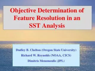
Objective Determination of Feature Resolution in an SST Analysis. Dudley B. Chelton (Oregon State University) Richard W. Reynolds (NOAA, CICS) Dimitris Menemenlis (JPL). Background. GHRSST (The Group for High Resolution SST) includes many high resolution SST analyses

E N D
Objective Determination of Feature Resolution in an SST Analysis Dudley B. Chelton (Oregon State University) Richard W. Reynolds (NOAA, CICS) Dimitris Menemenlis (JPL)
Background • GHRSST (The Group for High Resolution SST) includes many high resolution SST analyses • There are differences in input data, grid resolution, and analysis procedures • There are differences in the feature resolution and noisiness in the various analyses • Reynolds and Chelton (2010, J. Climate) compared 6 SST analyses for 2006-08 to try to identify analysis problems and determine whether any of the analyses are superior . . . .
SST Analyses in the Gulf Stream Region 1 January 2007 • RSS OI • ~1/11°grid • NCEP RTG-HR • 1/12°grid • UK OSTIA • 1/20°grid • NCDC Daily OI: (AMSR + AVHRR) • 1/4°grid • Differences near the coast can exceed 5°C • Resolution of the Gulf Stream differs for all three analyses
SST Analyses in the Gulf Stream Region 1 January 2007 • RSS OI • ~1/11°grid • NCEP RTG-HR • 1/12°grid • UK OSTIA • 1/20°grid • NCDC Daily OI: (AMSR + AVHRR) • 1/4°grid • RSS and RTG-HR have about the same grid spacing but radically different feature resolution • OSTIA has 5x the grid resolution of NCDC, but is smoother
Conclusions from Reynolds and Chelton (2010) • There is no clear correlation between feature resolution and the grid resolution of the SST analysis • GHRSST and other analysis producers tend to emphasize grid resolution over feature resolution. • Users are misled and/or misunderstand the distinction. • If the analysis procedure pushes the feature resolution beyond the spatial and temporal resolution limitations of the data that go into the analysis, apparent small-scale features in the SST analysis can just be spurious noise • Can we objectively determine the feature resolution for an SST analysis?
Approach: Experiments with Synthetic Data Analyze the complete SST fields produced by an ocean general circulation model on a high-resolution grid over a given time period. Consider these fields to be the true SST Sub-sample these “true” SST fields at the times and locations of actual satellite observations Use the complete (referred to here as Full) and sub-sampled (referred to here as Reduced) SST fields as “data” for input to the same analysis procedure. Compare the SST analyses based on the Full and the Reduced SST data sets to assess the loss of feature resolution from: the analysis procedure data gaps
Source of “True” SST: The ECCO-2 Model 1/16o Ocean General Circulation Model ECCO-2 (Estimating the Circulation and Climate of the Ocean, Phase II) Horizontal grid : 6.9 km at equator; 4.9 km at 45° latitude Use daily averages of model SST for the 1-year period 1993 Use spatial and temporal sampling of AMSR and Pathfinder AVHRR data (both day and night) for the 1-year period 2004 Note: Only the times and locations of AMSR and AVHRR data are used – the actual satellite measurements of SST are NOT used For simulated high-res AVHRR data, linearly interpolate model SST to Pathfinder v5 grid (4.8 km at equator) For simulated low-res AMSR data, smooth model SST to 50 km and average on 1/4° grid (27.8 km at equator)
Two Stages Stage 2: Daily OI on 4.8 km grid Stage 1: Daily OI on 28 km grid
SST “Data”, 1 July 1993 • Top 2 panels: Simulated Low-Resolution Data • Small differences between Reduced (left) and Full sampling (right) • Bottom 2 panels: Simulated High-Resolution Data: • Large differences between Reduced (left) and Full sampling (right) • The Low- and High-Resolution fields with Full sampling are visibly different (top & bottom right)
SST Hi-Res Reduced “Data”, 1 July 1993 • Our focus is on the spatial variance as a function of wavenumber (the reciprocal of the wavelength, λ) for 2 regions: • Gulf Stream • Sargasso Sea • Zonal Wavenumber spectra were computed for: • Each of 31 daily maps along zonal line at center of the box • These 31 spectra were then averaged
Gulf Stream Auto-Spectra, July 1993 • Linear Horizontal Axis • Wavenumber range 0-0.1 km-1, which corresponds to a wavelength range of λ > 10 km • Log vertical axis • Spectral density in powers of 10 • 3-days of hi-res “data” with full coverage • Spectrum drops steeply by 6 orders of magnitude • Spectrum is roughly flat for λ < 12.5 km • This flattening is due to interpolation from the model grid to the Pathfinder v5 “data” grid. λ = 100 km λ = 10 km λ = 20 km
Gulf Stream Auto-Spectra, July 1993 • The 3 curves are: • “Data” Hi-Res Full • OI Low-Res Full • OI Low-Res Reduced • The two OI Low-Res versions are indistinguishable • This shows that the low-res scales are adequately resolved by the sampling in the reduced data • Both OI Low-Res are much less energetic than the “data” • Factor of ~10 smaller at a wavelength λ=100 km • Factor of ~104 smaller at wavelengths λ< 50 km λ = 100 km λ = 10 km λ = 20 km
Gulf Stream Auto-Spectra, July 1993 • Add 2 more curves: OI Hi-Res Full OI Hi-Res Reduced • Both are very similar to Data at wavelengths λ>30 km • OI Hi-Res Full is less energetic than “Data” at shorter wavelengths due to the filtering in the OI procedure • OI Hi-Res Reduced is actually more energetic than “Data” at wavelengths λ<20 km The added energy at short wavelengths is purely noise!!! λ = 100 km λ = 10 km λ = 20 km
Gulf Stream Squared Coherence (γ2), July 1993(Coherence is the correlation as a function of wavenumber,λ-1) • Coherences were computed between analyses and “Data” Hi-Res Full: • OI Hi-Res Full • γ2 > 0.9 for all wavelengths • OI Low-Res Reduced • γ2 ~ 0.6 at λ=100 kmand drops to zero for λ < 50 km • OI Hi-Res Reduced • γ2 only slightly better than OI Low-Res Reduced • This verifies that the high wavenumber energy in OI Hi-Res Reduced is just noise λ = 100 km λ = 10 km λ = 20 km
Sargasso Sea Squared Coherence (γ2), July 1993 • OI Hi-Res Full • γ2 > 0.95 for λ > 20 kmand then drops gradually to ~0.5 for λ < 14 km • OI Low-Res Reduced • γ2 ~ 0.5 at λ=100 kmand drops to zero for λ < 75 km • OI Hi-Res Reduced is somewhat better than the Gulf Stream region because of better data distribution • γ2 decreases approximately linearly to ~0.1 at λ=20 km • No significant γ2 for λ < 20 km λ = 100 km λ = 10 km λ = 20 km
Gulf Stream (left) & Sargasso (right)Daily Coherence vs. Fractional Coverage • X axis: Daily Fractional Coverage: (Ocean Regions with Data)/(Total Regions) • Y axis: Daily Average Coherence in the wavenumber range 0.02 - 0.04 cpkm-1 (wavelength range 50 - 25 km) averaged along 31 zonal lines in each region • Coherence γ2is approximately proportional to Fractional Coverage • Fractional coverage is much better for Sargasso Sea than for the Gulf Stream, hence higher resolution SST analyses are possible
Numbers of 50% Coverage Days in January and July 2004 • Number of days with at least 50% ocean grid points with data • Computed on 1o spatial grid • January - top • July - bottom • Note strong seasonal differences, e.g., • Gulf Stream • N. Hem Indian Ocean • Eastern Tropical Pacific • This provides a qualitative way to assess: • Where high resolution analysis is possible • How often it is possible Number of Days
Summary • Using “Synthetic SST Data” as “Truth” is a useful procedure for studying the effects of sampling errors on SST analyses • Note that noise has not be added to the model SST in the simulations presented here • These high-resolution simulations are therefore optimistic • Monthly maps of data coverage provide a useful way for users to understand where and how often high-resolution analyses have reliable small-scale features • User must decide on desired accuracy (coherence level), which is approximately linearly related to the fractional coverage, e.g., γ2 >0.5 => 50% coverage
What is an Analysis? • An analysis is a field produced on a regular grid ( ) usually using irregularly spaced data • The data ( , ) are weighted by distance to the analysis point and by a noise-to-signal ratio
Input SST Data • In situ data: directly measured SST observations from ships and buoys • Remotely sensed satellite Infrared SSTs • 1-9 km resolution • Observations must be cloud free • e.g., AVHRR (1981-present) • Remotely sensed satellite Microwave SSTs • 50 km resolution • Observations can be made through clouds but must be precipitation free • e.g., AMSR (2002-present)
Results Daily low- and high-resolution OI run for a 1-year period using complete "data" coverage (full) and data subsampled to simulate actual satellite data coverage (reduced) Because of limited high resolution coverage due to clouds, 3-day spans of low- and high-resolution data were used for each daily analysis Two periods were considered: 1993 model output using 2004 satellite data coverage Products to be examined Low-resolution data-only (3days): Full & Reduced Low-resolution OI analysis: Full & Reduced High-resolution data-only (3 days): Full & Reduced High-resolution OI analysis: Full & Reduced
SST Analyses in the Western Tropical Pacific 1 January 2007 • RSS OI • (~1/11)° grid • NCEP RTG-HR • (1/12)°grid • UK OSTIA • (1/20)°grid • NCDC Daily OI: (AMSR + AVHRR) • (1/4)°grid • These are daily averages • What feature scales are justified based on the input data?
Gulf Stream (left) & Sargasso (right)Daily 1993 Coherence vs. Fractional Coverage • Daily Fractional Coverage: (Ocean Regions with Data)/(Total Regions) • Daily Average Coherence: (0.02-0.04 cpkm-1) or (50-25 km wavelength) averaged along 31 zonal lines symmetric about the central zonal line in the box • Coherence roughly proportional to Fractional Coverage • Fractional coverage is much better for Sargasso Sea than for the Gulf Stream