Modern Planning Techniques Part II
650 likes | 871 Vues
Modern Planning Techniques Part II. Jőrg Hoffmann Albert-Ludwigs-University Freiburg, Germany. Outline. Modern Planners (since 1995) Part I: ID PLANMIN Reachability Regression Search Non-directional Search Part II: Greedy PLANSAT Ignoring Delete Lists Local Search Topology

Modern Planning Techniques Part II
E N D
Presentation Transcript
Modern Planning TechniquesPart II Jőrg Hoffmann Albert-Ludwigs-University Freiburg, Germany
Outline • Modern Planners (since 1995) • Part I: ID PLANMIN • Reachability • Regression Search • Non-directional Search • Part II: Greedy PLANSAT • Ignoring Delete Lists • Local Search Topology • Numeric and Temporal Extensions • Summary
Greedy PLANSAT Directly consider plan existence problem, without plan length bound Greedy element: simply assume that there is a plan, and (heuristically) go look for (an arbitrary)one + we can use non-admissible heuristics – techniques (per se) completely useless for proving unsolvability, or finding provably optimal plans
FF vs. IPP in Gripper ([Helmert 03]: most benchmarks have lower complexity in sub-optimal case)
Part II: Greedy PLANSAT • Ignoring Delete Lists • A Popular Relaxation • Approximating Relaxed Plan Length • Heuristic Search • Systems, and Open Questions • Local Search Topology • Heuristic Landscapes • h+ in the Planning Benchmarks • Open Questions
Relaxations • General principle for deriving heuristics: Define a simplification (aka relaxation) of the problem, take solution to the simplified problem as heuristic • Eg, straight-line distance as a heuristic in a road map is based on the simplification that one needs no roads • Eg, k-reachability is based on the simplification that we only need to achieve the hardest k-subset • Another possible relaxation in planning: ignore the negative effects (aka delete lists) of the operators
Ignoring Delete Lists • Technically: pre => add, del pre => add • Example Drive-truck: at(T,L1) => at(T,L2), ¬at(T,L1) • Set of true facts increases monotonically under relaxed action application • Simplifies task because preconditions and goals are all positive
Example T P1 P2 • Relaxed Plan: Load T P1 Left Drive T Left Right Unload T P1 Right Load T P2 Right Unload T P2 Left
Ignoring Delete Lists, ctd. • We focus on sequential plans in the following, more generally on action count heuristics • Optimal relaxed plan length is an admissible heuristic Bylander [94]: relaxed PLANSAT is in P, relaxed PLANMIN is NP-complete => Use approximations of optimal relaxed plan length to obtain, in general non-admissible, heuristics • Percentage of domain-independent competition planners using this idea: 20%'98, 42%'00, 63%'02 => ??% '04
Relaxed Plan Length • Say we want to know, in the current search state, the number of actions needed to get from fact set F to fact set F' (concrete search schemes: see below) • Admissible estimate: h+(F,F') := length of optimal (shortest) relaxed plan from F to F' • h+ hard to compute => we approximate
Forward Chaining • Bonet & Geffner [97,99,01]: (HSP1/2, HSPr) h(F,f) := 0, if fF; else, mina,fadd(a) (1+ppre(a) h(F,p)) h(F,F') := fF'h(F,f) • ie, estimate „cost“ of fact set by sum of fact costs • Assumes that facts must be achieved independently • ignores positive interactions • can overestimate
Forward Chaining, ctd. • For all f : h(F,f) := 0, if fF; h(F,f) := ∞, else • While ( changes occured ) • for all a, ppre(a) h(F,p) < ∞: for all f, fadd(a): h(F,f ) := min(h(F,f ), 1+ ppre(a) h(F,p)) • Note: • this is a value iteration technique... • we might have to re-compute this for each state, depending on the search scheme (see later)
Example T P1 P2 • Fact costs: (F = initial state, F' = goal) • at(T,Left) 0, at(P1,Left) 0, at(P2,Right) 0 • at(T,Right) 1, in(P1,T) 1 • at(P1,Right) 3, in(P2,T) 2 • at(P2,Left) 3 • h+(F,F') = 5; h(F,F') = 6(Drive T Left Right counted twice)
Backward Chaining • McDermott [96,99]: (Unpop) „Greedy Regression-Match Graphs“ • Roughly: • start with single open subgoal F' • regress (ignoring interactions) each open subgoal O through all action sets A s.t. reg(O,A) F is maximal • leaf nodes are O F • cost of leaf O is 0, else it‘s minA (|A| +cost of reg(O,A))
Example T P1 P2 • Backwards graph: (F = initial state, F' = goal) • at(P1,Right), at(P2,Left) • Unload T P1 Right, Unload T P2 Left • in(P1,T), at(T,Right), in(P2,T) • Load T P1 Left, Drive T Left Right, Load T P2 Right -- OR ... • at(T,Right) • Drive T Left Right • h+(F,F‘) = 5; h(F,F‘) = 6 (Drive T Left Right counted twice)
Backward Chaining, ctd. • Computing greedy regression-match graphs appears to be very time-consuming • Can ignore positive interactions • Refanidis & Vlahavas [99,01]: (GRT) „Greedy Regression Tables“ • If F' is constant during search, one can partly pre-compute the backchaining process (see later) • …and take some positive interactions into account
Fwd./Bwd. Chaining • Hoffmann & Nebel [00,01]: (FF) Chain forward to compute fact costs; use fact costs for efficient backward chaining • Chain forward to compute parallel reachability in the relaxation (one can simply replace HSP-“” by “max”) • Chain backwards in reachability layers, and select achieving actions below • Is the same as a relaxed Graphplan execution, returns a relaxed plan
Example, Fwd. T P1 P2 • Fact costs: (F = initial state, F' = goal) • at(T,Left) 0, at(P1,Left) 0, at(P2,Right) 0 • at(T,Right) 1, in(P1,T) 1 • at(P1,Right) 2, in(P2,T) 2 • at(P2,Left) 3 • Iterations == relaxedplanning graph layers
Example, Bwd. T P1 P2 • Backwards action selection: (F = initial state, F' = goal) • 3: at(P2,Left) • Unload T P2 Left • 2: at(P1,Right), in(P2,T) • Unload T P1 Right, Load T P2 Right • 1: in(P1,T), at(T,Right) • Load T P1 Left, Drive T Left Right • Iterations == relaxed regression
SearchSchemes • Search Scheme (S, s0, br, Sol): • space of all search states S • start state s0S • branching rule br:S ((S)) (maps a state to a set of branching points; each branching point is a set of search states) • solution states Sol S (s.t. below each branching point there are the same solutions) • Transition-cost c:S x S N0, path-cost g(s0 ... s) • Remaining cost heuristic h: S N0 ? Heuristic search algorithm? • In what follows, branching heuristic not considered; we simply assume a set of successors to each state
Forward Search • Search Scheme (S, s0, br, Sol) where • S == space of all fact sets F, ie world states • s0 == initial state • br(s) == a single branching point, containing the results of executing the actions (or parallel action sets) applicable in F • Sol == fact sets that contain the goal • c(s,s') here, uniform 1, ie action count (step count) • Easy to understand, captures reachability; needs to be informed about relevance
Backward/Regression Search • Search Scheme (S, s0, br, Sol) where • S == space of all fact sets F, ie sub-goals • s0 == original goal set • br(s) == a single branching point, containing F‘s regression through all possible actions (or parallel action sets) • Sol == fact sets contained in original initial state • c(s,s') here, uniform 1, ie action count (step count) • Captures relevance; needs to be informed about reachability (in particular, “spurious” states are possible)
Partial-Order Search • Search Scheme (S, s0, br, Sol) where • S == space of all partially ordered ID‘ed actions • s0 == ({0:aI, 1:aG}, {0<1}) where aI/aG are dummy actions that add the initial state/require the goal • br(s) == branching points are the flaws (open conditions or threats), each point contains the set of possible flaw repairs • Sol == search states without flaws • c(s,s') here, 1 if flaw repair added an action, 0 else (ie action count) • More flexible than either forward or backward search, maybe better for temporal planning; captures relevance, spurious states possible • Branching heuristics known as „flaw selection strategies“
From F to F' • The semantics: • In forward search, F is the current search state, and F' is the goal • In backward search, F is the initial state, and F' is the current subgoal • In partial-order search, F is the initial state and F' are the currently open conditions • If F' is the same throughout search then heuristic backchaining can be (partially) pre-computed GRT • If F is the same throughout search then heuristic forward chaining can be (partially) pre-computed HSP
Global Search Algorithms Expand all search states in an order that depends on their heuristic values • Weighted A*: combine path costs and remaining costs by f(s) := w * g(s) + (1-w) * h(s) and expand search states by increasing f value • First found solution optimal (wrptoc) if w = 0.5, and heuristic admissible (wrptoc) (valid irrespective of branching heuristic) (eg. partial order) • Greedy with w < 0.5, extreme case w = 0,Best-first search, used in many planners
Local Search Algorithms Look at local surroundings of search states, and try to make improvements on h value • Hill-climbing: • Start in s0 • When in s, select one successor s' s.t. h(s') minimal • „Enforced Hill-climbing“: (used in FF) • Start in s0 • When in s, do breadth-first search for s' s.t. h(s') < h(s) • Note: algorithms of this kind can‘t prove unsolvability
Systems, Overview STAN4, LPG, AltAlt „special cases“...
Systems • Unpop [McDermott]: fwd search, bwd h, best-first/hill-climbing • HSP1 [Bonet&Geffner]: fwd search, fwd h, hill-climbing • HSPr [Bonet&Geffner]: bwd search, fwd h (pre-computation), best-first • GRT [Refanidis&Vlahavas]: fwd search, bwd h (pre-computation), best-first • FF [Hoffmann&Nebel]: fwd search, fwd/bwd h, enforced hill-climbing/best-first; pruning technique using relaxed plans • HSP2 [Bonet&Geffner]: configurable; fwd search, fwd h, best-first • AltAlt [Kambhampati et.al.]: bwd search, fwd h (various versions, including non-relaxed plan based ones), weighted A*
Systems, ctd. • Mips [Edelkamp&Helmert]: hybrid; fwd search, fwd/bwd h, weighted A* • STAN4 [Fox&Long]: hybrid; fwd search, fwd/bwd henhanced with generic types-knowledge, hill-climbing • Repop [Nguyen&Rao]: partial-order search, fwd/bwd h, weighted A* • SAPA [Do&Rao]: temporal&numeric; fwd search, fwd/bwd h, weighted A* • VHPOP [Younes&Simmons]: partial-order search, fwd h, weighted A* • LPG [Gerevini&Serina&al.]: search in the space of „action graphs“ (partial planning graphs); amongst others, a heuristic extracting relaxed plans for preconditions in the planning graph (fwd/bwd in that sense); hill-climbing style algorithm • Metric-FF [Hoffmann]: relaxation extended to numeric variables
Open Questions (I) How can we develop heuristics that yield good performance in those cases where current planners are bad? • Improve on relaxed plan estimate using additional information (STAN4, LPG) • Use different relaxations (eg pattern databases [Edelkamp 01])
Open Questions (II) How can we speed up the computations that estimate relaxed plan length in each search state? • Bottleneck in most systems (easily 80% of runtime) • Remove actions that are irrelevant within relaxation [Hoffmann&Nebel 01] • Re-use computation made in previous search state [Liu et al 02] • Avoid operator instantiation?
.bbl • T.Bylander. The Computational Complexity of Propositional STRIPS Planning. AIJ’94. • D.McDermott, A Heuristic Estimator for Means-Ends Analysis in Planning. AIPS’96. • B.Bonet, H.Geffner, Planning as Heuristic Search. AI’01. • I.Refanidis, I.Vlahavas, GRT: A Domain-Independent Heuristic for STRIPS Worlds Based on Greedy Regression Tables. ECP’99. • J.Hoffmann, B.Nebel, The FF Planning System: Fast Plan Generation Through Heuristic Search. JAIR’01. • M. Fox, D. Long, STAN4: A Hybrid Planning Strategy Based on Subproblem Abstraction. AIM’01. • X.Nguyen, S.Kambhampati, Reviving Partial Order Planning. IJCAI‘01 • M.Do, S.Kambhampati, Sapa: A Domain-Independent Heuristic Metric Temporal Planner. ECP’01.
.bbl, ctd. • X.Nguyen, S. Kambhampati, Extracting Effective and Admissible State Space Heuristics from the Planning Graph. AAAI’00. • J.Hoffmann, Extending FF to Numerical State Variables. ECAI’02. • H.Younes, R. Simmons, On the Role of Ground Actions in Refinement Planning. AIPS’02. • A. Gerevini, A. Saetti, I. Serina, Planning through Stochastic Local Search and Temporal Action Graphs in LPG. JAIR’03. • S.Edelkamp, Planning with Pattern Databases. ECP’01. • J.Hoffmann, B.Nebel, RIFO Revisited: Detecting Relaxed Irrelevance. ECP’01. • Y.Liu, S.Koenig, D.Furcy, Speeding Up the Calculation of Heuristics for Heuristic-Search-Based Planning. AAAI’02. • M. Helmert, Complexity Results for Standard Benchmark Domains in Planning, AIJ’03.
Heuristic Quality => Search Performance • A common-sense wisdom: The performance of a heuristic search algorithm is largely determined by the quality of the heuristic function • Extreme cases: + h(s) exact -- solution is found in linear time –h(s) constant -- no heuristic information, search trivializes to breadth/depth-first
Problem Structure => Heuristic Quality • Another common-sense wisdom: The quality of a heuristic function is largely determined by the structure of the specific problem instance • Extreme cases: + when driving X-over is possible, straight-line distance is exact – eg, getting from Hurghada to Sharm-el-Sheik
Local Search Topology • Search space with heuristic forms a landscape: states, and state transitions == road map heuristic values == height of states • Heuristic search moves along this landscape, searching for a lowest point (== solution) • Measure heuristic quality by form of landscape, its “local search topology” • Formally, landscape is annotated directed graph • Eg, [Frank et. al., JAIR-97] (for random SAT)
Local Minima “Must go upwards to reach a solution“
Local Minima Maximal exit distance Exit “Must go upwards to reach a solution“
Benches “All neighbour states look the same“
Benches Exit Maximal exit distance Exit “All neighbour states look the same“
Dead Ends “There is no path to a solution“
Unrecognised Dead Ends Recognised “There is no path to a solution“
Local Search Topology in Planning Benchmarks • We look at: (1)forward state space search (2)with the h+ heuristic • Why (1)? – simple to look at,used in many systems (in particular, my own) • Why (2)? – approximated by state-of-the-art sytems, can obtain hard(provable) results for it
A Planning Domain Taxonomy:(proved) Topology under h+ In lowermost classes, FF‘s search algorithm is polynomial!
Structure => Topology • There are 3 widely spread patterns of structure: Pattern 1 => no dead ends Patterns 1 & 2 => no local minima Patterns 1 & 2 & 3 => maximal benchexit distance <= c
Patterns of Structure - I • (At least) invertible actions: actions a to which there exists an inverse action undoing (at least) a‘s effects • Irrelevant negative effects: not needed anywhere • Static add effects: not deleted by any action • Example: • Drive T Left Right / Drive T Right Left • Load / Unload
Patterns of Structure - II • Actions that are respected by the relaxation: if a starts an optimal plan from (any) s, then a also starts an optimal relaxed plan from s (=> construct relaxed plan for successor state by either removing a, or replacing it with the inverse action) • Example: • Drive T Left Right: truck is needed at right side, to load/unload package • Load T P1 Left: P1 must be at right side • Unload T P1 Left: P1 must be at left side
Patterns of Structure - III • Actions whose negativeeffects are irrelevant upon execution: once a has been applied on an optimal solution path, a‘s negative effects are no longer needed (neither real nor relaxed) • Example: • Load T P1 Left: P1 must be at right side, delete is at(P1 Left) • Unload T P1 Left: P1 must be at left side, delete is in(P1 T) • Other actions (example: Drive) need to be applied on an optimal solution path <= c times in a row (example: 1)
Structure => Topology Pattern I Patterns I&II Patterns I&II&III
Open Questions (I) Is this (the quality of h+) a good or a bad result for AI planning? • Are the observed patterns of structure a phenomenon of the real world, or only a phenomenon of the, unrealistically simple, benchmarks? • Hard to answer, just like that. Best, get more realistic benchmarks