Ch 5.4: Regular Singular Points
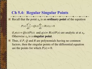
Ch 5.4: Regular Singular Points. Recall that the point x 0 is an ordinary point of the equation if p ( x ) = Q ( x )/ P ( x ) and q ( x )= R ( x )/ P ( x ) are analytic at at x 0 . Otherwise x 0 is a singular point .

Ch 5.4: Regular Singular Points
E N D
Presentation Transcript
Ch 5.4: Regular Singular Points • Recall that the point x0 is an ordinary point of the equation if p(x) = Q(x)/P(x) and q(x)= R(x)/P(x) are analytic at at x0. Otherwise x0 is a singular point. • Thus, if P, Q and R are polynomials having no common factors, then the singular points of the differential equation are the points for which P(x) = 0.
Example 1: Bessel and Legendre Equations • Bessel Equation of order : • The point x = 0 is a singular point, since P(x) = x2is zero there. All other points are ordinary points. • Legendre Equation: • The points x = 1 are singular points, since P(x) = 1- x2is zero there. All other points are ordinary points.
Solution Behavior and Singular Points • If we attempt to use the methods of the preceding two sections to solve the differential equation in a neighborhood of a singular point x0, we will find that these methods fail. • This is because the solution may not be analytic at x0, and hence will not have a Taylor series expansion about x0. Instead, we must use a more general series expansion. • A differential equation may only have a few singular points, but solution behavior near these singular points is important. • For example, solutions often become unbounded or experience rapid changes in magnitude near a singular point. • Also, geometric singularities in a physical problem, such as corners or sharp edges, may lead to singular points in the corresponding differential equation.
Numerical Methods and Singular Points • As an alternative to analytical methods, we could consider using numerical methods, which are discussed in Chapter 8. • However, numerical methods are not well suited for the study of solutions near singular points. • When a numerical method is used, it helps to combine with it the analytical methods of this chapter in order to examine the behavior of solutions near singular points.
Solution Behavior Near Singular Points • Thus without more information about Q/P and R/P in the neighborhood of a singular point x0, it may be impossible to describe solution behavior near x0. • It may be that there are two linearly independent solutions that remain bounded as x x0; or there may be only one, with the other becoming unbounded as x x0; or they may both become unbounded as x x0. • If a solution becomes unbounded, then we may want to know if y in the same manner as (x- x0)-1 or |x- x0|-½, or in some other manner.
Example 1 • Consider the following equation whichhas a singular point at x = 0. • It can be shown by direct substitution that the following functions are linearly independent solutions, for x 0: • Thus, in any interval not containing the origin, the general solution is y(x) = c1x2 + c2x-1. • Note that y = c1x2 is bounded and analytic at the origin, even though Theorem 5.3.1 is not applicable. • However, y = c2x-1 does not have a Taylor series expansion about x = 0, and the methods of Section 5.2 would fail here.
Example 2 • Consider the following equation which has a singular point at x = 0. • It can be shown the two functions below are linearly independent solutions and are analytic at x= 0: • Hence the general solution is • If arbitrary initial conditions were specified at x= 0, then it would be impossible to determine both c1 and c2.
Example 3 • Consider the following equation which has a singular point at x = 0. • It can be shown that the following functions are linearly independent solutions, neither of which are analytic at x = 0: • Thus, in any interval not containing the origin, the general solution is y(x) = c1x-1 + c2x-3. • It follows that every solution is unbounded near the origin.
Classifying Singular Points • Our goal is to extend the method already developed for solving near an ordinary point so that it applies to the neighborhood of a singular point x0. • To do so, we restrict ourselves to cases in which singularities in Q/P and R/P at x0 are not too severe, that is, to what might be called “weak singularities.” • It turns out that the appropriate conditions to distinguish weak singularities are
Regular Singular Points • Consider the differential equation • If P and Q are polynomials, then a regular singular point x0is singular point for which • For more general functions than polynomials, x0is a regular singular point if it is a singular point with • Any other singular point x0is an irregular singular point.
Example 4: Bessel Equation • Consider the Bessel equation of order • The point x = 0 is a regular singular point, since both of the following limits are finite:
Example 5: Legendre Equation • Consider the Legendre equation • The point x = 1 is a regular singular point, since both of the following limits are finite: • Similarly, it can be shown that x = -1 is a regular singular point.
Example 6 • Consider the equation • The point x = 0 is a regular singular point: • The point x = 2, however, is an irregular singular point, since the following limit does not exist:
Example 7: Nonpolynomial Coefficients(1 of 2) • Consider the equation • Note that x = /2 is the only singular point. • We will demonstrate that x = /2 is a regular singular point by showing that the following functions are analytic at /2:
Example 7: Regular Singular Point(2 of 2) • Using methods of calculus, we can show that the Taylor series of cosx about /2 is • Thus which converges for all x, and hence is analytic at /2. • Similarly, sinx analytic at /2, with Taylor series • Thus/2 is a regular singular point of the differential equation.