The L-E (Torque) Dynamical Model:
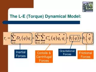
The L-E (Torque) Dynamical Model:. Gravitational Forces. Inertial Forces. Coriolis & Centrifugal Forces. Frictional Forces. Lets Apply the Technique -- . Lets do it for a 2-Link “Manipulator”. Link 1 has a Mass of m1; Link 2 a mass of m2. Before Starting lets define a L-E Algorithm:.

The L-E (Torque) Dynamical Model:
E N D
Presentation Transcript
The L-E (Torque) Dynamical Model: Gravitational Forces Inertial Forces Coriolis & Centrifugal Forces Frictional Forces
Lets Apply the Technique -- Lets do it for a 2-Link “Manipulator” Link 1 has a Mass of m1; Link 2 a mass of m2
We Start with Ai’s Not Exactly D-H Legal (unless there is more to the robot than these 2 links!)
So Let’s find T02 • T02= A1*A2
I’ll Compute Similar Terms back – to – back rather than by the Algorithm
Finding D1 • Consider each link a thin cylinder • These are Inertial Tensors with respect to a Fc aligned with the link Frames at the Cm
Finishing J1 Note the 2nd column is all zeros – even though Joint 2 is revolute – this is the special case!
Jumping into J2 This is 4th column of A1
Developing the D(q) Contributions • D(q)I = (Ai)TmiAi + (Bi)TDiBi • Ai is the “Upper half” of the Ji matrix • Bi is the “Lower Half” of the Ji matrix • Di is the Normalized Inertial Tensor of Linki defined in the Base space but acting on the link end
Building D(q)1 • D(q)1 = (A1)Tm1A1 + (B1)TD1B1 • Here:
Looking at the 2nd Term (Angular Velocity term) • Recall that D1 is: • Then:
Building the Full Manipulator D(q) • D(q)man= D(q)0 + D(q)1+ D(q)2 • Where • D(q)2 = (A2)Tm2A2+ (B2)TD2B2 • And recalling (from J2):
Building the 2rd D(q)2 Term: • Recall D2(nor. In.Tensor): • Then:
Simplifying then D(q) is: NOTE: D(q)man is Square in the number of Joints!
This Completes the Fundamental Steps: • Now we compute the Velocity Coupling Matrix and Gravitation terms:
Plugging ‘n Chugging • From Earlier: • THUS:
Finding h1: • Given: gravity vector points in –Y0direction (remembering the model!) • gk =(0, -g0, 0)T • g0is the gravitational constant • In the ‘h’ model Akij is extracted from the relevant Jacobianmatrix (– for Joint i) • Here:
Continuing: Note: Only k = 2 has a value for gk which is -g0!
Building “Torque” Models for each Link • In General:
For Link 1: • The 1st terms: • 2nd Terms:
Ist 2 terms: • 1st Terms: • 2nd Terms: