Download
1 / 45
450 likes | 521 Vues
Learn about the standard Normal Distribution, 68-95-99.7 Rule, calculations, and properties of normal curves.

E N D
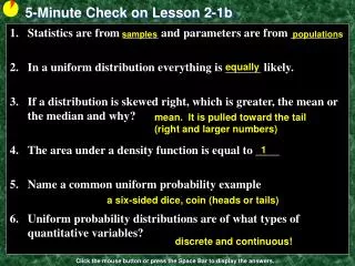
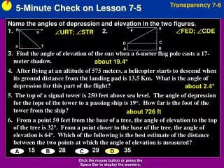
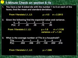
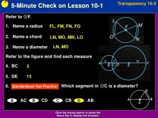
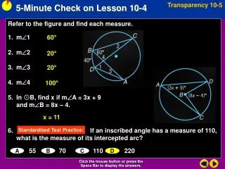
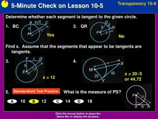
5-Minute Check on Lesson 2-1b Statistics are from ______ and parameters are from ________ In a uniform distribution everything is ______ likely. If a distribution is skewed right, which is greater, the mean or the median and why? The area under a density function is equal to ____ Name a common uniform probability example Uniform probability distributions are of what types of quantitative variables? samples populations equally mean. It is pulled toward the tail (right and larger numbers) 1 a six-sided dice, coin (heads or tails) discrete and continuous! Click the mouse button or press the Space Bar to display the answers.
Lesson 2 - 2 Normal Distributions
Objectives • DESCRIBE and APPLY the 68-95-99.7 Rule • DESCRIBE the standard Normal Distribution • PERFORM Normal distribution calculations • ASSESS Normality
Vocabulary • 68-95-99.7 Rule (or Empirical Rule) – given a density curve is normal (or population is normal), then the following is true:within plus or minus one standard deviation is 68% of datawithin plus or minus two standard deviation is 95% of datawithin plus or minus three standard deviation is 99.7% of data • Inverse Normal – calculator function that allows you to find a data value given the area under the curve (percentage) • Normal curve – special family of bell-shaped, symmetric density curves that follow a complex formula • Standard Normal Distribution – a normal distribution with a mean of 0 and a standard deviation of 1
Normal Curves • Two normal curves with different means (but the same standard deviation) [on left] • The curves are shifted left and right • Two normal curves with different standard deviations (but the same mean) [on right] • The curves are shifted up and down
Normal Density Curve Properties • It is symmetric about its mean, μ • Because mean = median = mode, the highest point occurs at x = μ • It has inflection points at μ – σ and μ + σ • Area under the curve = 1 • Area under the curve to the right of μ equals the area under the curve to the left of μ, which equals ½ • As x increases or decreases without bound (gets farther away from μ), the graph approaches, but never reaches the horizontal axis (like approaching an asymptote) • The Empirical Rule (68-95-99.7) applies
Empirical Rule μ ± 3σ μ ± 2σ μ ± σ 99.7% 95% 68% 2.35% 2.35% 34% 34% 0.15% 0.15% 13.5% 13.5% μ - 2σ μ μ + 2σ μ - 3σ μ - σ μ + σ μ + 3σ Normal Probability Density Function 1 y = -------- e √2π -(x – μ)2 2σ2 where μ is the mean and σ is the standard deviation of the random variable x
Area under a Normal Curve The area under the normal curve for any interval of values of the random variable X represents either • The proportion of the population with the characteristic described by the interval of values or • The probability that a randomly selected individual from the population will have the characteristic described by the interval of values [the area under the curve is either a proportion or the probability]
Standardizing a Normal Random Variable X - μ Z statistic: Z = ----------- σ where μ is the mean and σ is the standard deviation of the random variable X Z is normally distributed with mean of 0 and standard deviation of 1 Note: we are going to use tables (for Z statistics) not the normal PDF!! Or our calculator (see next chart)
Example 1 A random variable x is normally distributed with μ=10 and σ=3. • Compute Z for x1 = 8 and x2 = 12 • If the area under the curve between x1 and x2 is 0.495, what is the area between z1 and z2? 8 – 10 -2 Z = ---------- = ----- = -0.67 3 3 12 – 10 2 Z = ----------- = ----- = 0.67 3 3 0.495
The Standard Normal Table • Because all Normal distributions are the same when we standardize, we can find areas under any Normal curve from a single table. • Definition:The Standard Normal Table • Table A is a table of areas under the standard Normal curve. The table entry for each value z is the area under the curve to the left of z. Suppose we want to find the proportion of observations from the standard Normal distribution that are less than 0.81. We can use Table A: P(z < 0.81) = .7910
Normal Distributions on TI-83 • normalpdfpdf = Probability Density FunctionThis function returns the probability of a single value of the random variable x. Use this to graph a normal curve.Using this function returns the y-coordinates of the normal curve. • Syntax: normalpdf (x, mean, standard deviation)taken from http://mathbits.com/MathBits/TISection/Statistics2/normaldistribution.htm • Remember the cataloghelp app on your calculator • Hit the + key instead of enter when the item is highlighted
Normal Distributions on TI-83 • normalcdf cdf = Cumulative Distribution FunctionThis function returns the cumulative probability from zero up to some input value of the random variable x. Technically, it returns the percentage of area under a continuous distribution curve from negative infinity to the x. You can, however, set the lower bound. • Syntax: normalcdf (lower bound, upper bound, mean, standard deviation)(note: lower bound is optional and we can use -E99 for negative infinity and E99 for positive infinity)
Normal Distributions on TI-83 • invNorminv = Inverse Normal PDFThis function returns the x-value given the probability region to the left of the x-value. (0 < area < 1 must be true.) The inverse normal probability distribution function will find the precise value at a given percent based upon the mean and standard deviation. • Syntax: invNorm (probability, mean, standard deviation)
Properties of the Standard Normal Curve • It is symmetric about its mean, μ = 0, and has a standard deviation of σ = 1 • Because mean = median = mode, the highest point occurs at μ = 0 • It has inflection points at μ – σ = -1 and μ + σ = 1 • Area under the curve = 1 • Area under the curve to the right of μ = 0 equals the area under the curve to the left of μ, which equals ½ • As Z increases the graph approaches, but never reaches 0 (like approaching an asymptote). As Z decreases the graph approaches, but never reaches, 0. • The Empirical Rule (68-95-99.7) applies
Calculate the Area Under the Standard Normal Curve • Three different area calculations • Find the area to the left of a value • Find the area to the right of a value • Find the area between two values • There are several ways to calculate the area under the standard normal curve • What does not work – some kind of a simple formula • We can use a table (such as Table IV on the inside back cover) • We can use technology (a calculator or software) • Using technology is preferred
Normal Distribution Calculations How to Solve Problems Involving Normal Distributions • State: Express the problem in terms of the observed variable x. • Plan: Draw a picture of the distribution and shade the area of interest under the curve. • Do: Perform calculations. • Standardizex to restate the problem in terms of a standard Normal variable z. • Use Table A and the fact that the total area under the curve is 1 to find the required area under the standard Normal curve. • Conclude: Write your conclusion in the context of the problem.
a a a b Obtaining Area under Standard Normal Curve
a Example 2 Determine the area under the standard normal curve that lies to the left of • Z = -3.49 • Z = -1.99 • Z = 0.92 • Z = 2.90 Normalcdf(-E99,-3.49) = 0.000242 Normalcdf(-E99,-1.99) = 0.023295 Normalcdf(-E99,0.92) = 0.821214 Normalcdf(-E99,2.90) = 0.998134
a Example 3 Determine the area under the standard normal curve that lies to the right of • Z = -3.49 • Z = -0.55 • Z = 2.23 • Z = 3.45 Normalcdf(-3.49,E99) = 0.999758 Normalcdf(-0.55,E99) = 0.70884 Normalcdf(2.23,E99) = 0.012874 Normalcdf(3.45,E99) = 0.00028
a b Example 4 Find the indicated probability of the standard normal random variable Z • P(-2.55 < Z < 2.55) • P(-0.55 < Z < 0) • P(-1.04 < Z < 2.76) Normalcdf(-2.55,2.55) = 0.98923 Normalcdf(-0.55,0) = 0.20884 Normalcdf(-1.04,2.76) = 0.84794
a a Example 5 Find the Z-score such that the area under the standard normal curve to the left is 0.1. Find the Z-score such that the area under the standard normal curve to the right is 0.35. invNorm(0.1) = -1.282 = a invNorm(1-0.35) = 0.385
Summary and Homework • Summary • All normal distributions follow empirical rule • Standard normal has mean = 0 and StDev = 1 • Table A gives you proportions that are less than z • Homework • Day 1: 41, 43, 45, 47, 49, 51
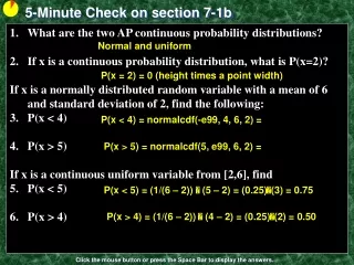
5-Minute Check on Lesson 2-2a What is the mean and standard deviation of Z? Given the following distributions: A~N(4,1), B~N(10,4) C~N(6,8) Which is the tallest? Which is the widest? The Empirical Rule is also known as the __ , __ , ___ rule. Given P(z < a) = 0.251, find P(z > a) In distribution B, what is the area to the left of 10? mean, = 0 and standard deviation, = 1 distribution A (it has smallest ) distribution C (it has largest ) 68 95 99.7 P( z > a) = 1 – P(z < a) = 1 – 0.251 = 0.749 0.5 (half area is to left of mean) Click the mouse button or press the Space Bar to display the answers.
Finding the Area under any Normal Curve • Draw a normal curve and shade the desired area • Convert the values of X to Z-scores using Z = (X – μ) / σ • Draw a standard normal curve and shade the area desired • Find the area under the standard normal curve. This area is equal to the area under the normal curve drawn in Step 1 • Using your calculator, normcdf(-E99,x,μ,σ)
Given Probability Find the Associated Random Variable Value Procedure for Finding the Value of a Normal Random Variable Corresponding to a Specified Proportion, Probability or Percentile • Draw a normal curve and shade the area corresponding to the proportion, probability or percentile • Use Table IV to find the Z-score that corresponds to the shaded area • Obtain the normal value from the fact that X = μ + Zσ • Using your calculator, invnorm(p(x),μ,σ)
Example 1 For a general random variable X with • μ = 3 • σ = 2 a. Calculate Z b. Calculate P(X < 6) Z = (6-3)/2 = 1.5 so P(X < 6) = P(Z < 1.5) = 0.9332 Normcdf(-E99,6,3,2) or Normcdf(-E99,1.5)
Example 2 For a general random variable X with μ = -2 σ = 4 • Calculate Z • Calculate P(X > -3) Z = [-3 – (-2) ]/ 4 = -0.25 P(X > -3) = P(Z > -0.25) = 0.5987 Normcdf(-3,E99,-2,4)
Example 3 For a general random variable X with • μ = 6 • σ = 4 calculate P(4 < X < 11) P(4 < X < 11) = P(– 0.5 < Z < 1.25) = 0.5858 Converting to z is a waste of time for these Normcdf(4,11,6,4)
Example 4 For a general random variable X with • μ = 3 • σ = 2 find the value x such that P(X < x) = 0.3 x = μ + Zσ Using the tables: 0.3 = P(Z < z) so z = -0.525 x = 3 + 2(-0.525) so x = 1.95 invNorm(0.3,3,2) = 1.9512
Example 5 For a general random variable X with • μ = –2 • σ = 4 find the value x such that P(X > x) = 0.2 x = μ + Zσ Using the tables: P(Z>z) = 0.2 so P(Z<z) = 0.8 z = 0.842 x = -2 + 4(0.842) so x = 1.368 invNorm(1-0.2,-2,4) = 1.3665
a b Example 6 • For random variable X with • μ = 6 • σ = 4 • Find the values that contain 90% of the data around μ x = μ + Zσ Using the tables: we know that z.05 = 1.645 x = 6 + 4(1.645) so x = 12.58 x = 6 + 4(-1.645) so x = -0.58 P(–0.58 < X < 12.58) = 0.90 invNorm(0.05,6,4) = -0.5794 invNorm(0.95,6,4) = 12.5794
Summary and Homework • Summary • Using a calculator we can avoid converting to z-values before calculating the area under the normal curves • Calculator gives you proportions between any two values (-e99 and e99 represent - and ) • Homework • Day 2: 53, 55, 57, 59
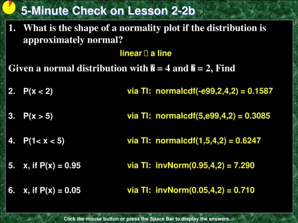
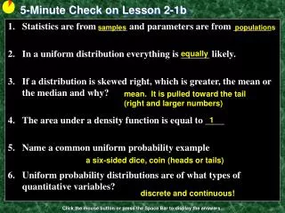
5-Minute Check on Lesson 2-2b Given a normal distribution with = 4 and = 2, Find P(x < 2) P(x > 5) P(1< x < 5) x, if P(x) = 0.95 x, if P(x) = 0.05 via TI: normalcdf(-e99,2,4,2) = 0.1587 via TI: normalcdf(5,e99,4,2) = 0.3085 via TI: normalcdf(1,5,4,2) = 0.6247 via TI: invNorm(0.95,4,2) = 7.290 via TI: invNorm(0.05,4,2) = 0.710 Click the mouse button or press the Space Bar to display the answers.
Is Data Normally Distributed? • For small samples we can readily test it on our calculators with Normal probability plots • Large samples are better down using computer software doing similar things
Normality Plots • Most software packages can construct Normal probability plots. These plots are constructed by plotting each observation in a data set against its corresponding percentile’s z-score. Interpreting Normal Probability Plots If the points on a Normal probability plot lie close to a straight line, the plot indicates that the data are Normal. Systematic deviations from a straight line indicate a non-Normal distribution. Outliers appear as points that are far away from the overall pattern of the plot.
TI-83 Normality Plots • Enter raw data into L1 • Press 2nd ‘Y=‘ to access STAT PLOTS • Select 1: Plot1 • Turn Plot1 ON by highlighting ON and pressing ENTER • Highlight the last Type: graph (normality) and hit ENTER. Data list should be L1 and the data axis should be x-axis • Press ZOOM and select 9: ZoomStat Does it look pretty linear? (hold a piece of paper up to it)
Non-Normal Plots • Both of these show that this particular data set is far from having a normal distribution • It is actually considerably skewed right
Example 1: Normal or Not? Roughly Normal (linear in mid-range) with two possible outliers on extremes
Example 2: Normal or Not? Not Normal (skewed right); three possible outliers on upper end
Example 3: Normal or Not? Roughly Normal (very linear in mid-range)
Example 4: Normal or Not? Roughly Normal (linear in mid-range) with deviations on each extreme
Example 5: Normal or Not? Not Normal (skewed right) with 3 possible outliers
Example 6: Normal or Not? Roughly Normal (very linear in midrange) with 2 possible outliers
Summary and Homework • Summary • Calculator gives you proportions between any two values (-e99 and e99 represent - and ) • Assess distribution’s potential normality by • comparing with empirical rule • normality probability plot (using calculator) • Homework • Day 3: 63, 65, 66, 68-74