5-Minute Check on section 7-1b

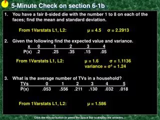
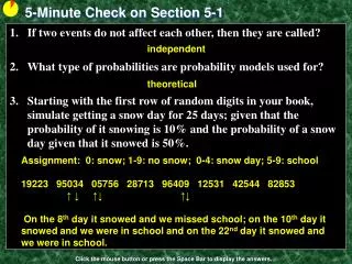
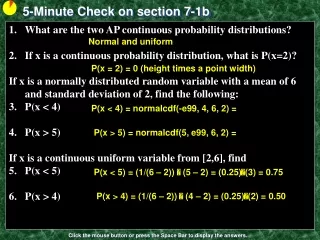
1. 5-Minute Check on section 7-1b What are the two AP continuous probability distributions? If x is a continuous probability distribution, what is P(x=2)? If x is a normally distributed random variable with a mean of 6 and standard deviation of 2, find the following: P(x < 4) P(x > 5) If x is a continuous uniform variable from [2,6], find P(x < 5) P(x > 4) Normal and uniform P(x = 2) = 0 (height times a point width) P(x < 4) = normalcdf(-e99, 4, 6, 2) = P(x > 5) = normalcdf(5, e99, 6, 2) = P(x < 5) = (1/(6 – 2))  (5 – 2) = (0.25)(3) = 0.75 P(x > 4) = (1/(6 – 2))  (4 – 2) = (0.25)(2) = 0.50 Click the mouse button or press the Space Bar to display the answers.

2. Lesson 7 – 2a Means and Variancesof Random Variables

3. Knowledge Objectives • Define what is meant by the mean of a random variable • Explain what is meant by a probability distribution • Explain what is meant by a uniform distribution • Discuss the shape of a linear combination of independent Normal random variables

4. Construction Objectives • Calculate the mean of a discrete random variable. • Calculate the variance and standard deviation of a discrete random variable. • Explain, and illustrate with an example, what is meant by the law of large numbers. • Explain what is meant by the law of small numbers. • Given µx and µy, calculate µa+bx, and µx+y. • Given x and y, calculate 2a+bx, and 2x+y (where x and y are independent). • Explain how standard deviations are calculated when combining random variables.

5. Vocabulary • Mean – balance point of the probability histogram or density curve. Symbol: μx • Standard Deviation – square root of the variance. Symbol: x • Variance – is the average squared deviation of the values of the variable from their mean. Symbol: σ²x

6. Means • Mean of a random variable is also known as its expected value

7. Discrete Random Variable - Mean The mean, or expected value [E(x)], of a discrete random variable is given by the formula μx = ∑ [x ∙P(x)] where x is the value of the random variable and P(x) is the probability of observing x Mean of a Discrete Random Variable Interpretation: If we run an experiment over and over again, the law of large numbers helps us conclude that the difference between x and ux gets closer to 0 as n (number of repetitions) increases

8. Variance

9. Discrete Random Variable - Variance Variance and Standard Deviation of a Discrete Random Variable: The variance of a discrete random variable is given by: σ2x = ∑ [(x – μx)2 ∙ P(x)] = ∑[x2 ∙ P(x)] – μ2x and standard deviation is √σ2 Note: round the mean, variance and standard deviation to one more decimal place than the values of the random variable

10. Uniform PDF An experiment is said to be a Uniform experiment provided: • The probability of each value of the random variable is equal (like in a six-sided die) • The trials are independent of each other (what happened last does not affect what happens next)

11. Uniform PDF If X is a value of the uniform random variable, then probability formula for X is 1 P(x) = ------- x = 0, 1, 2, 3, … , n n where n is the total number of discrete values of the random variable x Mean: μx = ∑ [x ∙P(x)] = (1/n)∑ x Standard Deviation: σ2x = ∑ [(x – μx)2 ∙ P(x)] = (1/n) ∑ [(x – μx)2 = ∑[x2 ∙ P(x)] – μ2x = (1/n) ∑ [x2 ] – μx2

12. Using your TI-83 calculator We can use 1-Var-Stats to calculate the mean and standard deviation of a discrete random variable given it’s outcomes and probability • Type in outcomes (x values) in L1 • Type in corresponding probabilities in L2 • Use 1-Var-Stats L1, L2 to get statistics We can graph the probability histograms by changing the frequency to L2

13. Example 1 You have a fair 10-sided die with the number 1 to 10 on each of the faces. Determine the mean and standard deviation. Mean: ∑ [x ∙P(x)] = (1/10) (∑ x) = (1/10)(55) = 5.5 Var: ∑[x2 ∙ P(x)] – μ2x = (1/n) ∑ [x2 ] – μx2 = (1/10) (385) - 30.25) = (38.5 – 30.25) = 8.25 St Dev = 2.8723

14. Example 2 Below is a distribution for number of visits to a dentist in one year.  X = # of visits to a dentist x 0 1 2 3 4 P(x) .1 .3 .4 .15 .05 Determine the expected value, variance and standard deviation. Mean: ∑ [x ∙P(x)] = (.1)(0) + (.3)(1) + (.4)(2) + (.15)(3) + (.05)(4) = 0 + .3 + .8 + .45 +.2 = 1.75 Var: ∑[x2 ∙ P(x)] – μ2x = ∑ [x2 ∙ P(x)] – μx2 = (0 + .3 + .4(4) + .15(9) + .05(16) ) – 3.0625) = 4.05 – 3.8626 = 0.9875 St Dev = 0.9937

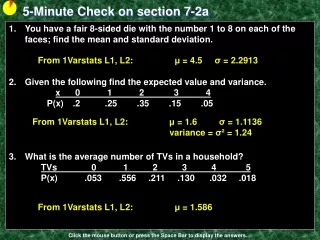
15. Example 3 What is the average size of an American family? Here is the distribution of family size according to the 1990 Census: # in family 2 3 4 5 6 7 p(x) .413 .236 .211 .090 .032 .018 Mean: ∑ [x ∙P(x)] = (.413)(2) + (.236)(3) + (.211)(4) + (.09)(5) + (.032)(6) + (.018)(7) = .826 + .708 + .844 + .45 + .192 + .126 = 3.146

16. Example 4 You are trying to decide whether to take out a $250 deductible which will cost you $90 per year. Records show that for this community the average cost of repair is $900. Records also show that 10% of the drivers have an accident during the year. If you have sufficient assets so that you will not be financially handicapped if you had to pay out the $900 or more for repairs, should you buy the policy? P(accident) = 0.1 so P(no accident) = 0.9ave repair cost = $900 Yearly cost = $90Expected Yearly with Policy: ∑ [x ∙P(x)] = (.1)(250) + (.9)(0) + 90 = 25 + 90 = $115 Expected Yearly without: ∑ [x ∙P(x)] = (.1)(900) + (.9)(0) = $90

17. Summary and Homework • Summary • Expected value is the mean ∑ [x ∙ P(x)] • Variance is ∑[x2 ∙ P(x)] – μ2x • Standard Deviation is variance • Use your calculator! • Homework • pg 486-7; 7.24 – 7.30