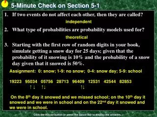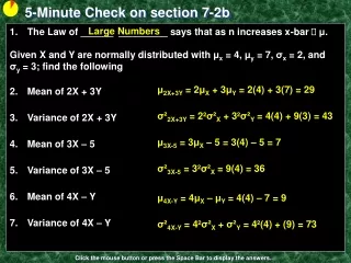
5-Minute Check on section 7-1a
120 likes | 141 Vues
Learn the basics of discrete and continuous random variables, probability rules, and probability terms, with examples and vocabulary. Understand the difference between qualitative and quantitative variables.

5-Minute Check on section 7-1a
E N D
Presentation Transcript
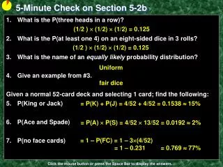
5-Minute Check on section 7-1a Convert these statements into discrete probability expressions Probability of less than 4 green bulbs Probability of more than 2 green lights Probability of 3 or more If x is a discrete variable x[1,3], P(x=1) = 0.23, and P(x=2) = 0.3 Find P(x<3) Find P(x=3) Find P(x>1) P(x < 4) = P(0) + P(1) + P(2) + P(3) P(x > 2) = P(3) + P(4) + P(5) + … P(x 3) = P(3) + P(4) + P(5) + … = P(1) + P(2) = 0.23 + 0.3 = 0.57 = 1 – (P(1) + P(2)) = 1 – 0.57 = 0.43 = P(2) + P(3) = 0.3 + 0.43 = 0.73 Click the mouse button or press the Space Bar to display the answers.
Lesson 7 – 1b Discrete and ContinuousRandom Variables
Objectives • Define statistics and statistical thinking • Understand the process of statistics • Distinguish between qualitative and quantitative variables • Distinguish between discrete and continuous variables
Vocabulary • Random Variable – a variable whose numerical outcome is a random phenomenon • Discrete Random Variable – has a countable number of random possible values • Probability Histogram – histogram of discrete outcomes versus their probabilities of occurrence • Continuous Random Variable – has a uncountable number (an interval) of random possible values • Probability Distribution – is a probability density curve
Probability Rules • 0 ≤ P(X) ≤ 1 for any event X • P(S) = 1 for the sample space S • Addition Rule for Disjoint Events: • P(A B) = P(A) + P(B) • Complement Rule: • For any event A, P(AC) = 1 – P(A) • Multiplication Rule: • If A and B are independent, then P(A B) = P(A)P(B) • General Addition Rule (for nondisjoint) Events: • P(E F) = P(E) + P(F) – P(E F) • General Multiplication rule: • P(A B) = P(A) P(B | A)
Probability Terms • Disjoint Events: • P(A B) = 0 • Events do not share any common outcomes • Independent Events: • P(A B) = P(A) P(B) (Rule for Independent events) • P(A B) = P(A) P(B | A) (General rule) • P(B) = P(B|A) (lines 1 and 2 implications) • Probability of B does not change knowing A • At Least One: • P(at least one) = 1 – P(none) • From the complement rule [ P(AC) = 1 – P(A) ] • Impossibility: P(E) = 0 • Certainty: P(E) = 1
Continuous Random Variables • Variable’s values follow a probabilistic phenomenon • Values are uncountable (infinite) • P(X = any value) = 0 (area under curve at a point) • Examples: • Plane’s arrival time -- minutes late (uniform) • Calculator’s random number generator (uniform) • Heights of children (apx normal) • Birth Weights of children (apx normal) • Distributions that we will study • Uniform • Normal
Continuous Random Variables • We will use a normally distributed random variable in the majority of statistical tests that we will study this year • Need to justify it (as a reasonable assumption) if is not given • Normality graphs if we have raw data • We need to be able to • Use z-values in Table A • Use the normalcdf from our calculators • Graph normal distribution curves
Example 4 Determine the probability of the following random number generator: • Generating a number equal to 0.5 • Generating a number less than 0.5 or greater than 0.8 • Generating a number bigger than 0.3 but less than 0.7 P(x = 0.5) = 0.0 P(x ≤ 0.5 or x ≥ 0.8) = 0.5 + 0.2 = 0.7 P(0.3 ≤ x ≤ 0.7) = 0.4
Example 5 In a survey the mean percentage of students who said that they would turn in a classmate they saw cheating on a test is distributed N(0.12, 0.016). If the survey has a margin of error of 2%, find the probability that the survey misses the percentage by more than 2% [P(x<0.1 or x>0.14)] Change into z-scores to use table A 0.10 – 0.12 z = ---------------- = +/- 1.25 0.016 0.8944 – 0.1056 = 0.7888 1 – 0.7888 = 0.2112 ncdf(0.1, 0.14, 0.12, 0.016) = 0.7887 1 – 0.7887 = 0.2112
Summary and Homework • Summary • Random variables (RV) values are a probabilistic • RV follow probability rules • Discrete RV have countable outcomes • Continuous RV has an interval of outcomes (∞) • Homework • Day 2: pg 475 – 476, 7.7, 7.8 pg 477 – 480, 7.11, 7.15, 7.17, 7.18