Superconducting Devices for Quantum Computation
Superconducting Devices for Quantum Computation. Xiangning Luo EE 698A Department of Electrical Engineering, University of Notre Dame. Outline of Presentation. Introduction to quantum computation Superconducting qubit devices Josephson charge qubit

Superconducting Devices for Quantum Computation
E N D
Presentation Transcript
Superconducting Devices for Quantum Computation Xiangning Luo EE 698A Department of Electrical Engineering, University of Notre Dame
Outline of Presentation • Introduction to quantum computation • Superconducting qubit devices • Josephson charge qubit • Qubits based on the flux degree of freedom
Quantum Computation Classical Computation: Classical logic bit: “0” and “1” Quantum Computation: Quantum bit, “Qubit”, can be manipulated using the rules of quantum physics Orthogonal quantum states |0> , |1> and their superposition |Ψ> = c0|0> + c1|1> A Quantum state of M bits is a superposition of 2M states. The quantum computation is a parallel computation in which all 2M basis vectors are acted upon at the same time. If one wanted to simulate a quantum computer using a classical computer one would need to multiply together 2M dimensional unitary matrices, to simulate each step. A quantum computer can factorize a 250-digit number in seconds while an ordinary computer will take 800 000 years!
Quantum Computation Preparation: The initial preparation of the state defines a wave function at time t0=0. 0 U(t1,t0) |Ψ(0)> |Ψ(1)> 1 U(t2,t1) State evolution: Evolved by a sequence of unitary operations …. U(tn,tn-1) |Ψ(n)> n Measurement: Quantum measurement is projective. Collapsed by measurement of the state P(Ф)=|<Ф|Ψ(n)>|2
Quantum Logic Gates Question: How to implement a general unitary operator? Answer: Introduce a complete set of logic gates. Any possible operation on an qubit register can be represented in terms of a suitable sequence of actions of such elementary logic gates It is proved that an arbitrary 2x2 unitary matrix may be decomposed as U = where α,β,ν, andδare real-valued.
Superconducting Qubit Devices Any quantum mechanically coherent system could be used to implement the ideas of quantum computation. - single photons - nuclear spins - trapped ions - superconductors Advantage of solid state implementations Possibility of a scalable implementation of the qubits Superconducting devices The minimum levels of decoherence among solid state implementations. A promising implementation of qubit. two kinds of qubit devices either based on charge or flux degrees of freedom.
The Cooper Pair Box Qubit System Hamiltonian Tunneling term Energy state of n Cooper pair A sudden square pulse is applied to the gate Vg The square gate pulse lasts for some time ∆t Vg returns to zero The probability that the state does not return to the ground state
The superconducting Flux Qubit Coherent time evolution between two quantum states was observed. antisymmetric superposition symmetric superposition clockwise Φ=h/4e anticlockwise Flux qubit consists of 3 Josephson junctions arranged in a superconducting loop. Two states carrying opposite persistent currents are used to represent |0> and |1>. External flux near half Φ0=h/2e is applied. A SQIUD is attached directly. MW line provides microwave current bursts inducing oscillating magnetic fields. Current line provides the measuring pulse and voltage line allows the readout of the switching pulse. I. Chiorescu et al., Science 299, 1869 (2003).
The superconducting Flux Qubit Measurements of two energy levels of qubit Qubit energy separation is adjusted by changing the external flux. Resonant absorption peaks/dips are observed. Dots are measured peak/dip positions obtained by varying frequency of MW pulse. The continuous line is a numerical fit giving an energy gap ∆ = 3.4 GHz in agreement of numerical simulations. I. Chiorescu et al., Science 299, 1869 (2003).
The superconducting Flux Qubit Different MW pulse sequences are used to induce coherent quantum dynamics of the qubit in the time domain. Rabi oscillations - when the MW frequency equals the energy difference of the qubit, the qubit oscillates between the ground state and the excited state. Resonant MW pulse of variable length with frequency F = E10 is applied. The pulse length defines the relative occupancy of the ground state and the excited state. The switching probability is obtained by repeating the whole sequence of reequilibration, microwave control pulses, and readout typically 5000 times. MW F = 6.6GHz MW power 0dbm, -6dbm, and -12dbm Linear dependence of the Rabi frequency on the MW amplitude, a key signature of the Rabi process. Decay times up to ~150 ns results in hundreds of coherent oscillations. I. Chiorescu et al., Science 299, 1869 (2003).