Download
1 / 16
160 likes | 295 Vues
Analysis of Circulation Patterns in Lake Michigan using SeaWiFS imagery. By Raghavendra S. Mupparthy and Carolyn J. Merry Department of Civil, Environmental Engineering and Geodetic Sciences, The Ohio State University, Columbus. Outline. Introduction to SeaWiFS. Our archival at GLFS (OSU).

E N D
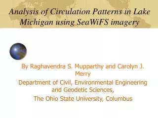
Analysis of Circulation Patterns in Lake Michigan using SeaWiFS imagery By Raghavendra S. Mupparthy and Carolyn J. Merry Department of Civil, Environmental Engineering and Geodetic Sciences, The Ohio State University, Columbus
Outline • Introduction to SeaWiFS. • Our archival at GLFS (OSU). • Lake Michigan Turbidity Study. • Goal of this talk. • Flow Chart of the process. • Results from SeaWiFS data analysis
705 km, noon, sun-synchronous orbit Ground IFOV at nadir = 1.1km Daily coverage Ground swath: GAC = 1502 km LAC = 2802 km 4 km resolution 1 km resolution Off nadir viewing + 20o Sea-viewing Wide Field-of-view Sensor (SeaWiFS)
Lake Michigan Statistics of Lake Michigan Length : 307 miles Width : 118 miles Maximum depth: 925 ft Average depth : 279 ft Shoreline: 1660 miles.
Turbidity Plume Event in Lake Michigan • For a decade, Lake Michigan has an episodic resuspension of turbidity - turbidity plume event. • It has been observed that the entire lake gets disturbed, and happens in the early spring. • Plume event is attributed to significant wind velocity fields over the lake.
Study Objective • Extract some measures for understanding the distribution of the suspended sediments. • Visualize this distribution with these parameters by comparing it with the previous years distribution to determine the change. • And check whether SeaWiFS can be used.
Chlorophyll A • CZCS Pigment Conc. • K-490 (Band 5/Band 1)* chloro_a(98) Methodology Level 2 0.89 Level 1 0.11 - = Change Binned image Base Image
Methodology The general approach adopted is • Process the Level – 1 SeaWiFS imagery in SeaDAS to get Level – 2 products. • Chlorophyll_a identified as the tracking agent. • Other potential tracking agents identified has been the level-2 k_490 product, CZCS pigment concentration product, and band ratio-ed image- band5/band1 and the reflectance data.
Results • An analytical model developed by Schwab et al on the turbidity plume event of 1998 indicated that – • There are 2 counter clock-wise rotating currents in the middle of the lake, clockwise gyre on the top and anti-clockwise in the southern part of the lake. • There is a deposition zone in between these two gyres.
SeaWiFS results, showing the pattern in the year 1998 Red color indicates more erosion, green is deposition and black is no change or negative from 1998
SeaWiFS results, showing the pattern in the year 1999 Red color indicates more erosion, green is deposition and black is no change or negative from 1998
SeaWiFS results, showing the pattern in the year 2000. Red color indicates more erosion, green is deposition and black is no change or negative from 1998
Conclusion • SeaWiFS can be used to study changes in the suspended material concentration in the Great Lakes. • Further work is needed to quantify this change in suspended sediment concentration
For further information - • For further information regarding the archival and the processed data, • http://hcgl.eng.ohio-state.edu/~seawifs • The data has been organized according to lake, year and month.