Download
1 / 31
350 likes | 826 Vues
Part B. Linear Algebra, Vector Calculus Chap. 6: Linear Algebra; Matrices, Vectors, Determinants, Linear Systems of Equations. Theory and application of linear systems of equations, linear transformations, and eigenvalue problems. - Vectors, matrices, determinants, …

E N D
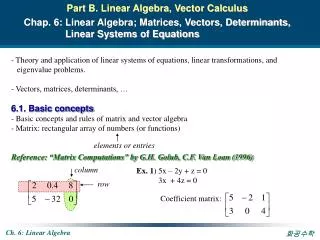
Part B. Linear Algebra, Vector Calculus Chap. 6: Linear Algebra; Matrices, Vectors, Determinants, Linear Systems of Equations • Theory and application of linear systems of equations, linear transformations, and • eigenvalue problems. • - Vectors, matrices, determinants, … • 6.1. Basic concepts • - Basic concepts and rules of matrix and vector algebra • - Matrix: rectangular array of numbers (or functions) • Reference: “Matrix Computations” by G.H. Golub, C.F. Van Loan (1996) elements or entries column Ex. 1) 5x – 2y + z = 0 3x + 4z = 0 row Coefficient matrix:
m x n matrix m = n: square matrix General Notations and Concepts aii: principal or main diagonal of the matrix. (important for simultaneous linear equations) Row (Eqn.) - rectangular matrix that is not square Column (Variable)
Vectors Row vector: Transposition Transpose Column vector: Symmetric matrices: Skew-symmetric matrices: Square matrices Properties of transpose:
Equalities of Matrices: same size • Matrix Addition: same size • Scalar Multiplication: • 6.2. Matrix Multiplication • Multiplication of matrices by matrices • (number of columns of 1st factor A = number of rows of 2nd factor B)
Difference from Multiplication of Numbers - Matrix multiplication is not commutative in general: - does not necessarily imply - does not necessarily imply (even when A=0) Special Matrices Upper triangular matrix Lower triangular matrix Banded matrix Results of finite difference solutions for PDE or ODE. (especially, tridiagonal) Matrix can be decomposed into Lower & Upper triangular matrices LU decomposition
Special Matrices: Diagonal matrix Symmetric matrix, Identity (or unit) matrix Inner Product of Vectors Product in Terms of Row and Column Vectors: (jth first row of A).(kth first column of B)
Linear Transformations • 6.3. Linear Systems of Equations: Gauss Elimination • The most important practical use of matrices: the solution of linear systems of equations • Linear System, Coefficient Matrix, Augmented Matrix b = 0: homogeneous system (this has at least one solution, i.e., x = 0) b 0: nonhomogeneous system Augmented matrix
x2 x1 Ex. 1) Geometric interpretation: Existence of solutions Precisely one solution Same slope Different intercept No solution Infinite solutions Very close to singular ill-conditioned - difficult to identify the solution - extremely sensitive to round-off error Singular
Gauss Elimination - Standard method for solving linear systems - The elimination of unknowns can be extended to large sets of equations. (Forward elimination of unknowns & solution through back substitution) During this operations the first row: pivot row (a11: pivot element) And then second row becomes pivot row: a’22 pivot element Repeat back substitution, moving upward Upper triangular form
Elementary Row Operation: Row-Equivalent Systems • - Interchange of two rows • Addition of a constant multiple of one row to another row • Multiplication of a row by a nonzero constant c • Overdetermined: equations > unknowns • Determined: equations = unknowns • Underdetermined: equations < unknowns • Consistent: system has at least one solution. • Inconsistent: system has no solutions at all. • Homogeneous solution: xh • Nonhomogeneous solution: xp • xp+xh is also a solutions of the nonhomogeneous systems • Homogeneous systems: always consistent (why? trivial solution exists, x=0) • Theorem: A homogeneous system possess nontrivial solutions if the number of m of • equations is less than the number of n of unknowns (m < n)
Echelon Form: Information Resulting from It (a) No solution: if r < m and one of the numbers is not zero. (b) Precisely one solution: if r=n and , if present, are zero. (c) Infinitely many solutions: if r < n and , if present, are zero. Existence and uniqueness of the solutions Next issue
Gauss-Jordan elimination: particularly well suited to digital computation Multiplying the second row by a’12 and subtracting the second row from the first - The most efficient approach is to eliminate all elements both above and below the pivot element in order to clear to zero the entire column containing the pivot element, except of course for the 1 in the pivot position on the main diagonal.
LU-Decomposition • Gauss elimination: • - Forward elimination + back-substitution • (computation effort ) • - Inefficient when solving equations with the same coefficient A, but with different rhs constants B • LU Decomposition: • - Well suited for those situations where many rhs B must be evaluated for a single value of A • Elimination step can be formulated so that it involves only operations on the matrix of coefficient A. • - Provides an efficient means to compute the matrix inverse. • (1) LU Decomposition • - LU decomposition separates the time-consuming elimination of A from the manipulations of rhs B. • once A has been “decomposed”, multiple rhs vectors can be evaluated effectively. • Overview of LU Decomposition • Upper triangular form: - Assume lower diagonal matrix with 1’s on the diagonal:
So that • - Two-step strategy for obtaining solutions: • LU decomposition step: A L and U • Substitution step: D from LD=B • x from Ux=D • LU Decomposition Version of Gauss Elimination • a. Gauss Elimination: • Use f21 = a21/a11 to eliminate a21 upper triangular matrix form ! • f31 = a31/a11 to eliminate a31 • f32 = a’32/a’22 to eliminate a32 • Store f’s
b. Forward-substitution step: Back-substitution step: (identical to the back-substitution phase of conventional Gauss elimination)
6.4. Rank of a Matrix: Linear Dependence. Vector Space - Key concepts for existence and uniqueness of solutions Linear Independence and Dependence of Vectors Given set of m vectors: a1, …, am (same size) Linear combination: (cj: any scalars) - Conditions satisfying above relation: (1) (Only) all zero cj’s: a1, …, am are linearly independent. (2) Above relation holds with scalars not all zero linearly dependent. Ex. 1) Linear independence and dependence - Vectors can be expressed into linearly independent subset. Two vectors are linearly independent.
Rank of a Matrix • - Maximum number of linearly independent row vectors of a matrix A=[ajk]: rank A • Ex. 3) Rank • rank = 2 • rank A=0 iff A=0 • Theorem 1: (rank in terms of column vectors) • The rank of a matrix A equals the maximum number of linearly independent column vectors of A. A and AT same rank. • Maximum number of linearly independent row vectors of A(r) cannot exceed the • maximum number of linearly independent column vectors of A. • Ex. 4)
Vector Space, Dimension, Basis • Vector space: a set V of vectors such that with any two vectors a and b in V all their • linear combination a+b are elements of V. • Let V be a set of elements on which two operations called vector addition and scalar multiplication are defined. Then V is said to be a vector space if the following ten properties are satisfied. • Axioms for vector addition • (i) If x and y are in V, then x+y is in V. • (ii) For all x, y in V, x+y = y+x • (iii) For all x, y, z in V, x+(y+z) = (x+y) +z • (iv) There is a unique vector 0 in V such that 0 + x = x + 0 = x • (v) For each x in V, there exists a vector –x such that x+(-x) = (-x)+x=0 • Axioms for scalar multiplications • (vi) If k is any scalar and x is in V, then kx is in V • (vii) k(x+y) = kx + ky • (viii) (k1+k2)x = k1x + k2x • (ix) k1(k2x) = (k1k2)x • (x) 1x = x
Vector Space, Dimension, Basis • Subspace: If a subset W of a vector space V is itself a vector space under the • operations of vector addition and scalar multiplication defined on V, then • W is called a subspace of V. • (i) If x and y are in W, then x+y is in W. • (ii) If x is in W and k is any scalar, then kx is W. • Dimension: (dim V) the maximum number of linearly independent vectors in V. • Basis for V: a linearly independent set in V consisting of a maximum possible • number of vectors in V. • (number of vectors of a basis for V = dim V) • Span: the set of linear combinations of given vectors a1, …, ap with the same number • of components (Span is a vector space) • Ex. 5) Consider a matrix A in Ex.1.: vector space of dim 2, basis a1, a2 or a1, a3 • Row space of A: span of the row vectors of a matrix A • Column space of A: span of the column vectors of a matrix A • Theorem 2: The row space and the column space of a matrix A have the same • dimension, equal to rank A.
Invariance of Rank under Elementary Row Operations • Theorem 3: Row-equivalent matrices • Row-equivalent matrices have the same rank. • (Echelon form of A: no change of rank property) • Ex. 6) • Practical application of rank in connection with the linearly independence and dependence of the vectors Theorem 4: p vectors x1, …, xp, (with n components) are linearly independent if the matrix with row vectors x1, …, xp has rank p: they are linearly dependent if that rank is less than p. Theorem 5: p vectors with n < p components are always linearly dependent. Theorem 6: The vector space Rn consisting of all vectors with n components has dimension n. rank A=2
6.5. Solutions of Linear Systems: Existence, Uniqueness, General Form Theorem 1: Fundamental theorem for linear systems (a) Existence: m equations in n unknowns has solutions iff the coefficient matrix A and the augmented matrix have the same rank. (b) Uniqueness: above system has precisely one solution iff this common rank r of A and equals n. (c) Infinitely many solutions: If rank of A = r < n, system has infinitely many solutions. (d) Gauss elimination: If solutions exist, they can all be obtained by the Gauss elimination.
The Homogeneous Linear System • Theorem 2: Homogeneous system • - A homogeneous linear system always has the trivial solution, x1=0,…, xn=0 • - Nontrivial solutions exist iff rank A<n. • If rank A=r<n, these solutions, together with x=0, form a vector space of dimension • n-r, called the solution space of above system. • - If x1 and x2 are solution vectors, then x=c1x1+c2x2 is also solution vector. • Theorem 3: A homogeneous linear system with fewer equations than unknowns • always has nontrivial solutions. • The Nonhomogeneous Linear System • Theorem 4: If a nonhomogeneous linear system of equations of the form Ax=b has • solutions, then all these solutions are of the form (x0 is any fixed solution of Ax=b, xh: solution of homogeneous system)
6.6. Determinants. Cramer’s Rule • Impractical in computations, but important in engineering applications (eigenvalues, • DEs, vector algebra, etc.) • - associated with an nxn square matrix • Second-order Determinants • Ex. 2) Cramer’s rule: • Third-order Determinants • Ex. 3) Cramer’s rule
Determinant of Any Order n Minor of ajk in D Cofactor of ajk in D Ex. 4) Third-order determinant
General Properties of Determinants Theorem 1: (a) Interchange of two rows multiplies the value of the determinant by –1. (b) Addition of a multiple of a row to another row does not alter the value of the determinant. (c) Multiplication of a row by c multiplies the value of the determinant by c. Ex. 7) Determinant by reduction to triangular form Theorem 2: (d) Transposition leaves the value of a determinant unaltered. (e) A zero row or column renders the value of a determinant zero. (f) Proportional rows or columns render the value of a determinant zero. In particular, a determinant with two identical rows or columns has the value zero.
General Properties of Determinants Theorem 1: (a) Interchange of two rows multiplies the value of the determinant by –1. (b) Addition of a multiple of a row to another row does not alter the value of the determinant. (c) Multiplication of a row by c multiplies the value of the determinant by c. Ex. 7) Determinant by reduction to triangular form Theorem 2: (d) Transposition leaves the value of a determinant unaltered. (e) A zero row or column renders the value of a determinant zero. (f) Proportional rows or columns render the value of a determinant zero. In particular, a determinant with two identical rows or columns has the value zero.
Rank in Terms of Determinants - Rank ~~~ determinants Theorem 3: An m x n matrix A=[ajk] has rank r1 iff A has an r x r submatrix with nonzero determinant, whereas the determinant of every square submatrix with r+1 or more rows that A has is zero. - If A is square, n x n, it has rank n iff det A0. Cramer’s Rule - Not practical in computations, but theoretically interesting in DEs and others Theorem 4: (a) Linear system of n equations in the same number of unknowns, x If this system has a nonzero coefficient determinant D=det A, it has precisely one solution.
(b) If the system is homogeneous and D0, it has only the trivial solution x=0. If D=0, the homogeneous system also has nontrivial solutions. 6.7. Inverse of a Matrix: Gauss-Jordan Elimination - If A has an inverse, then A is a nonsingular matrix (unique inverse !) ~~ no inverse, ~~ a singular matrix. Theorem 1: Existence of the inverse The inverse A-1 of an n x n matrix A exists iff rank A=n, hence iff det A0. Hence A is nonsingular if rank A = n, and is singular if rank A < n. Determination of the Inverse - n x n matrix A n x n identity matrix I, I matrix A-1
Matrix Inverse • a. Calculating the inverse • - The inverse can be computed in a column-by-column fashion • by generating solutions with unit vectors as the rhs constants. • resulting solution will be • the first column of the matrix inverse. • … the second column of the matrix inverse • Best way: use the LU decomposition algorithm • (evaluate multiple rhs vectors) • b. Matrix inversion by Gauss-Jordan elimination • The square matrix A-1 assumes the role of the column vector of unknown x, while square matrix I assumes the role of the rhs column vector B.
Some Useful Formulas for Inverse • Theorem 2: The inverse of a nonsingular n x n matrix A=[ajk] is given by • where Ajk is the cofactor of ajk in det A. • Ex. 3) For 3 x 3 matrix • Diagonal matrices A have an inverse iff all ajj0. Then A-1 is diagonal with entries • 1/a11, …, 1/ann. • Ex. 4) Inverse of a diagonal matrix • -
Vanishing of Matrix Products. Cancellation Law - Matrix multiplication is not commutative in general: - does not necessarily imply - does not necessarily imply (even when A=0) Theorem 3: Cancellation law Let A, B, C be n x n matrices. Then (a) If rank A=n and AB=AC, thenB=C (b) If rank A=n, then AB=0 implies B=0. Hence if AB=0, but A0 as well as B0, then rank A < n and rank B < n. (c) If A is singular, so are BA and AB. Determinants of Matrix Products Theorem 4: For any n x n matrices A and B