Download
1 / 29
290 likes | 555 Vues
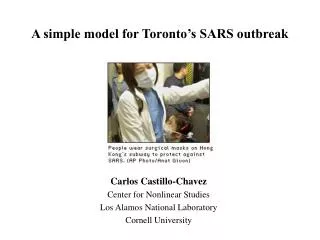
A simple model for Toronto’s SARS outbreak. Carlos Castillo-Chavez Center for Nonlinear Studies Los Alamos National Laboratory Cornell University. Outline. SARS epidemiology and related issues SARS transmission model (SEIJR) Parameter estimation and data fitting

E N D
A simple model for Toronto’s SARS outbreak Carlos Castillo-Chavez Center for Nonlinear Studies Los Alamos National Laboratory Cornell University
Outline • SARS epidemiology and related issues • SARS transmission model (SEIJR) • Parameter estimation and data fitting • The basic reproductive number • Simulation Results • Conclusions • Extensions and related models
SARS epidemiology and related issues • SARS (Severe Acute Respiratory Syndrome) is a new respiratory disease which was first identified in China’s southern province of Guangdong in November 2002. • The most striking feature of SARS is its ability to spread on a global scale. One man with SARS made 7 flights: from Hong Kong to Munich to Barcelona to Frankfurt to London, back to Munich and Frankfurt before finally returning to Hong Kong. • An individual exposed to SARS may become infectious after an incubation period of 2-7 days with 3-5 days being most common. • Most infected individuals either recover after 7-10 days or suffer 7% - 10% mortality. SARS appears to be most serious in people over age 40 especially those who have other medical problems.
SARS epidemiology and related issues, Cont’ • Researchers in the Erasmus medical center in Rotterdam recently demonstrated that a corona virus is the causative agent of SARS. • The mode of transmission is not very clear. SARS appears to be transmitted mainly by person-to-person contact. However, it could also be transmitted by contaminated objects, air, or by other unknown ways. Recently, it has been suggested that SARS’ corona virus may have come from an animal reservoir. • Presently there is no vaccine available. Rapid diagnosis and isolation of infectious individuals is critical for many reasons.
SARS transmission model • U.S. data is limited and sparsely distributed while the quality of China’s data is hard to evaluate. • There appears to be enough data for Toronto, Hong Kong and Singapore (WHO, Canada Ministry of Health) to build a preliminary model (single outbreak). • Single outbreak model ignores demographic processes other than the impact of SARS on survival.
S1 R E I J D k S2 C Compartmental model The model considers two distinct susceptible classes: S1, the most susceptible, and S2. is the transmission rate to S1from E, I and J. E is the class composed of asymptomatic, possibly infectious individuals. The class I denotes infected, symptomatic, infectious, and undiagnosed individuals. J are diagnosed individuals.
Initially S1 = and S2 = where is a fraction of the population at major risk of SARS infection and N is the total population. We can write the following system of ODE-s:
Parameter estimation and data fitting • The transmission rate was obtained from the initial rate of exponential growth r (computed from time series data). • The values of p and q are fixed arbitrarily while l and are varied and optimized (least squares criterion) for Toronto, Hong Kong and Singapore. • Some restrictions apply. For example: and Members of the diagnosed class J recover at the same rate as members of the undiagnosed class I. • All other parameters are taken from the current literature.
Basic reproductive number R0 The number of secondary infectious individuals generated by a single “typical” infectious individual when introduced into a population of only susceptible individuals. R0 =1.2 (Hong Kong and Toronto) R0 =1.1 (Singapore)
Basic Reproductive Number R0 =1.2 (Hong Kong and Toronto) R0 =1.1 (Singapore)
Initial Rates of Growth • Initial rates of growth r are computed from data provided by the WHO and the Canada Ministry of Health. These rates are computed exclusively from the cumulative number of cases reported between March 31 and April 14. • The values obtained are 0.0405 (world data), 0.0496 (Hong Kong) , 0.054 (Toronto) and 0.037 (Singapore). Start of the Outbreaks • Estimates of the start of the outbreaks in Toronto, Hong Kong and Singapore are obtained from the formula That is, we assume an initial exponential growth (r is the “model-free” rate of growth from the time series x(t) of the cumulative number of SARS cases).
The case of Toronto • The total population in Ontario is approximately 12 million. However, the population at major risk of SARS infection lives in the southern part which is approximately 40% of the total population ( in our model). • Hospital closures (Scarborough Grace hospital on March 25th and York Central hospital on March 28th), the jump in the reported number of Canadian SARS cases on March 31st and the rapid rise in recognized cases in the following week, indicate that doctors were rapidly diagnosing pre-existing cases of SARS (in either E or I on March 26th). At this point the diagnosis and isolation rates were changed:
Simulation results • (circles) data • (lines) cumulative number of SARS cases C • Prior to March 26: = 1/6, l=0.76 • The fit to data is given by = 1/3, l=0.05 (rapid diagnosis and effective isolation of diagnosed cases, dashed line) • The second curve is given by = 1/6, l=0.05 (slow diagnosis and effective isolation of diagnosed cases, dotted line) • The third curve is given by = 1/3, l=0.3 (rapid diagnosis with improved but imperfect isolation, dash-dot line)
Simulation results, Cont’ l =0.38 (Hong Kong) and l=0.4 (Singapore). Singapore has =0.68. All other parameters are from Table 1. The data is fitted starting March 31st because of the jump in reporting on March 30th.
Conclusions • By examining two cases with relatively clean exponential growth curves we are able to calibrate the SEIJR model. We use the model to study the non-exponential dynamics of the Toronto Outbreak after intervention. Two features of the Toronto data, the steep increase in the number of recognized cases after March 31st and the rapid slowing in the growth of new recognized cases, robustly constrain the SEIJR model by requiring that and days-1. • The fitting of data shows that initial rates of SARS growth are quite similar in most regions leading to estimates of R0 between 1.1 and 1.2.
Conclusions, cont’ • Both good isolation and rapid diagnosis are required for control. • In our model "good control" means (a) at least a factor of 10 reduction in l (effectiveness of isolation) and (b) simultaneously a maximum diagnostic period of 3 days. The model is sensitive to these parameters, so they should be treated as absolutely minimal requirements: better is better. • Although our work doesn't give us a technical basis for the following statement, it is reasonable to speculate that these (necessary) drastic isolation measure could bog down medical services and create huge expense for those who have to implement them (particularly if there is a delay in implementation). It will help the situation enormously if it becomes possible to rapidly diagnose SARS cases with a laboratory test: then many of the people with suspected SARS would only need to be isolated on a precautionary basis until the test results were in. The folks developing the test should have the maximum usable resources thrown at them.
EXTENSIONS/THOUGHTS • Transportation Systems • Transient Populations
NSU NSU SU SU Subway SU SU NSU NSU Subway Transportation Model
Proportionate mixing (Mixing Axioms) (1) Pij >0 (2) (3) ci Ni Pij = cj Nj Pji Then is the only separable solution satisfying (1) , (2), and (3).
Definitions the mixing probability between non-subway users from neighborhood i given that they mixed. the mixing probability of non-subway and subway users from neighborhood i, given that they mixed. the mixing probability of subway and non-subway users from neighborhood i, given that they mixed. the mixing probability between subway users from neighborhood i, given that they mixed. the mixing probability between subway users from neighborhoods i and j, given that they mixed. the mixing probability between non-subway users from neighborhoods i and j, given that they mixed. the mixing probability between non-subway user from neighborhood i and subway users from neighborhood j, given that they mixed.
Formulae of Mixing Probabilities (depends on activity level and allocated time)
Forthcoming BookMathematical and Modeling Approaches in Homeland Security SIAM's, Frontiers in Applied Mathematics Edited by Tom Banks and Carlos Castillo-Chavez , On sale on June 2003.