Calibration Techniques
Calibration Techniques. 1. Calibration Curve Method 2. Standard Additions Method 3. Internal Standard Method. Calibration Curve Method. Most convenient when a large number of similar samples are to be analyzed. Most common technique. Facilitates calculation of Figures of Merit.

Calibration Techniques
E N D
Presentation Transcript
Calibration Techniques 1. Calibration Curve Method 2. Standard Additions Method 3. Internal Standard Method
Calibration Curve Method Most convenient when a large number of similar samples are to be analyzed. Most common technique. Facilitates calculation of Figures of Merit.
Calibration Curve Procedure Prepare a series of standard solutions (analyte solutions with known concentrations). Plot [analyte] vs. Analytical Signal. Use signal for unknown to find [analyte].
Example: Pb in Blood by GFAAS Results of linear regression: S = mC + b m = 5.56 mAbs/ppb b = 0.93 mAbs
A sample containing an unknown amount of Pb gives a signal of 27.5 mAbs. Calculate the Pb concentration. S = mC + b C = (S - b) / m C = (27.5 mAbs – 0.92 mAbs) / 5.56 mAbs / ppb C = 4.78 ppb (3 significant figures)
Calculate the LOD for Pb 20 blank measurements gives an average signal 0.92 mAbs with a standard deviation of σbl = 0.36 mAbs LOD = 3 σbl/m = 3 x 0.36 mAbs / 5.56 mAbs/ppb LOD = 0.2 ppb (1 significant figure)
Find the LDR for Pb Lower end = LOD = 0.2 ppb (include this point on the calibration curve) SLOD = 5.56 x 0.2 + 0.93 = 2.0 mAbs (0.2 ppb , 2.0 mAbs)
Find the LDR for Pb Upper end = collect points beyond the linear region and estimate the 95% point. Suppose a standard containing 18.5 ppb gives rise to s signal of 98.52 mAbs This is approximately 5% below the expected value of 103.71 mAbs (18.50 ppb , 98.52 mAbs)
Find the LDR for Pb LDR = 0.2 ppb to 18.50 ppb or LDR = log(18.5) – log(0.2) = 1.97 2.0 orders of magnitude or 2.0 decades
Find the Linearity Calculate the slope of the log-log plot
Remember S = mC + b log(S) = log (mC + b) b must be ZERO!! log(S) = log(m) + log(C) The original curve did not pass through the origin. We must subtract the blank signal from each point.
Standard Addition Method Most convenient when a small number of samples are to be analyzed. Useful when the analyte is present in a complicated matrix and no ideal blank is available.
Standard Addition Procedure Add one or more increments of a standard solution to sample aliquots of the same size. Each mixture is then diluted to the same volume. Prepare a plot of Analytical Signal versus: volume of standard solution added, or concentration of analyte added.
Standard Addition Procedure The x-intercept of the standard addition plot corresponds to the amount of analyte that must have been present in the sample (after accounting for dilution). The standard addition method assumes: the curve is linear over the concentration range the y-intercept of a calibration curve would be 0
Example: Fe in Drinking Water The concentration of the Fe standard solution is 11.1 ppm All solutions are diluted to a final volume of 50 mL
[Fe] = ? x-intercept = -6.08 mL Therefore, 10 mL of sample diluted to 50 mL would give a signal equivalent to 6.08 mL of standard diluted to 50 mL. Vsam x [Fe]sam = Vstd x [Fe]std 10.0 mL x [Fe] = 6.08 mL x 11.1 ppm [Fe] = 6.75 ppm
Internal Standard Method Most convenient when variations in analytical sample size, position, or matrix limit the precision of a technique. May correct for certain types of noise.
Internal Standard Procedure Prepare a set of standard solutions for analyte (A) as with the calibration curve method, but add a constant amount of a second species (B) to each solution. Prepare a plot of SA/SB versus [A].
Notes The resulting measurement will be independent of sample size and position. Species A & B must not produce signals that interfere with each other. Usually they are separated by wavelength or time.
Example: Pb by ICP Emission Each Pb solution contains 100 ppm Cu.