Calibration
Ron Maddalena NRAO – Green Bank July 2009. Calibration. Receiver calibration sources allow us to convert the backend’s detected voltages to the intensity the signal had at the point in the system where the calibration signal is injected.

Calibration
E N D
Presentation Transcript
Ron Maddalena NRAO – Green Bank July 2009 Calibration
Receiver calibration sources allow us to convert the backend’s detected voltages to the intensity the signal had at the point in the system where the calibration signal is injected.
Determining TCal from hot-cold load measurements in the lab • Place black bodies (absorbers) of two known temperatures in front of the feed and record detected voltages. • VHot_Off = g * THot • VCold_Off = g * TCold • VCold_On = g * (TCold + TCal) • g and TCal are unknown
Determining TCal from hot-cold load measurements in the lab • Course frequency resolution • Uncertainties in load temperatures • Are the absorbers black bodies? • Detector linearities (300 & 75 K) • Lab TCal may be off by 10% • So… all good observers perform their own astronomical calibration observation
Continuum - Point SourcesOn-Off Observing • Observe blank sky for 10 sec • Move telescope to object & observe for 10 sec • Move to blank sky & observe for 10 sec • Fire noise diode & observe for 10 sec • Observe blank sky for 10 sec
Known: Equivalent temperature of noise diode or calibrator (Tcal) = 3 K Bandwidth (Δν) = 10 MHz Gain = 2 K / Jy Desired: Antenna temperature of the source (TA) Flux density (S) of the source. System Temperature(Ts) when OFF the source Accuracy of antenna temperature (σ TA) Continuum - Point SourcesOn-Off Observing
Units of “intensity” • TA is usually not a unit with much scientific interest. Need to correct for: • Lost power due to… • Earth’s atmosphere at the observing elevation. • Telescope efficiencies • Rayleigh-Jeans approximation may not be appropriate for your high-frequency observations • Shape of the telescope beam Shape of source.
Correcting for atmosphere and efficiencies • TR* -- secondary focus • TA* -- primary focus • Sometimes shortened to:
Telescope efficiencies – Part 2 • Aperture efficiency • At low frequencies: ηSurf = 1 • Almost always: ηr = 1 • For GBT, ηfss and ηl > 0.98 • All may be dependent upon frequency and observing elevation (Gain or Efficiency curve)
Shape of the telescope beam Shape of source. • Ta, Tr, etc. will be different for different telescopes for the same sky position.
To wink or not to wink? • Reminder – diode used to measure the gain and, thus, to calibrate from V to TA. • GBT – traditionally winks diode when on source • Tracks fast gain changes • Slightly easier to reduce • Adds to Tsys during all your observations • More time to achieve the desired sensitivity • Always observing the source • Arecibo – traditionally performs separate calibration observation off the source • Adds extra time to your observation • tracks gain changes less often
To wink or not to wink? – Spectral Line • Should wink if 1/f gain changes will add baseline structure >10 sec for z=2.5 CO(J=1-0) at Ka-band • The shorter the scan, the more likely winking will require less telescope time. <103-104 sec for galactic & extragalactic HI. Assumes 1% calibration, Tsys/Tcal = 10
Spectral Line Calibration • Today’s line observations should be treated like yesterday’s continuum observations • Weak wide lines with wide bandwdiths • High-Z CO lines • 30 MHz line widths • 14 GHz of bandwidth @ 30 GHz.
Raw Data Reduced Data – High Quality Reduced Data – Problematic
Spectral Line Calibration • Difference experiments • Position switching • Frequency witching • Nutating secondaries • Dual-beam systems: • Nodding telescope’s position • Nodding optics • Multi-feed systems • Atmosphere is common to all receivers (atmosphere is in the near field)
Traditional calibration algorithms • Good for narrow-band observations or strong lines when baseline structures aren’t important. • Not good for wide band work • Tsys and Tcal have frequency structure • Any difference in power between Sig and Ref will produce baseline structueres that are mirrors of the frequency structures inn Tsys and Tcal
Wide-bandwidth calibration • Same equations but with different averaging • Vector Tcal calibration • Identical to the equation used in the exercise for continuum observation • Not yet incorporated into the official GBTIDL release.