0 10 20 30 40 50 60 70 80 90 100
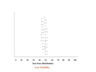
* * * * *. * * * * *. * * * * *. * * * * *. * * * * *. * * * * *. * * * * *. * * * * *. * * * * *. 0 10 20 30 40 50 60 70 80 90 100. Test Score Distribution.

0 10 20 30 40 50 60 70 80 90 100
E N D
Presentation Transcript
* * * * * * * * * * * * * * * * * * * * * * * * * * * * * * * * * * * * * * * * * * * * * 0 10 20 30 40 50 60 70 80 90 100 Test Score Distribution Low Variability
Positively Skewed Distribution Negatively Skewed Distribution 40 45 55 60 70 75 80 90 100 40 45 55 60 70 75 80 90 100 Test Scores Test Scores
Normal Curve -4 -3 -2 -1Mean +1 +2 +3 +4 Central Tendency a) Mode (most frequent score) b) Mean (average score; [EX/N]) c) Median (midpoint of scores) Variability (Spread in Scores) a) Range (lowest to highest score) b) Standard Deviation c) Variance
Computation of Standard Deviation & Variance Deviation scores (scores minus the mean Squared deviation scores Test Scores X 10 20 30 40 50 -20 -10 0 10 20 x x2 400 100 0 100 400 EX2 = 1000 (Sum of the squared deviation scores) EX = 150 (EX/N) = 30 (Mean) Mean of the sum of the squared deviation scores EX2/N = 200 (the variance or s2) = standard deviation or s s2 200 = 14.14 (standard deviation)
Relationships Among Different Types of Test Scores in a Normal Distribution Number of Cases 2.14% 0.13% 0.13% 2.14% 13.59% 34.13% 34.13% 13.59% -4 -3 -2 -1 Mean +1 +2 +3 +4 Test Score Z score T score CEEB score Deviation IQ (SD = 15) Stanine Percentile -4 -3 -2 -1 0 +1 +2 +3 +4 10 20 30 40 50 60 70 80 90 200 300 400 500 600 700 800 55 70 85 100 115 130 145 4% 7% 12% 17% 20% 17% 12% 7% 4% 1 2 3 4 5 6 7 8 9 1 5 10 20 30 40 50 60 70 80 90 95 100
85 84 83 82 81 80 79 78 77 76 75 74 73 72 71 70 69 68 67 66 65 64 63 62 61 60 * * * * * * * * * * * * * * * * * * * * * * * * * * * * * * * * * * * * * * * * * * * * * * * * * * * * * * * * Son’s Height 60 61 62 63 64 65 66 67 68 69 70 71 72 73 74 75 76 77 78 79 80 81 82 83 84 85 Fathers Height (in inches)
CORRELATION --- Some Key Concepts • Consists of a Set of Ordered Pairs • Indicates both the magnitude and direction of the relationship between variables • c) Range is from -1.0 to + 1.0
85 84 83 82 81 80 79 78 77 76 75 74 73 72 71 70 69 68 67 66 65 64 63 62 61 60 * * * * * * * * * * * Positive Correlation * * * * Job Performance * * * * * * * * * * * * * * * * * * * * * * * * * * * * * * * * * * * * * * * * * 60 61 62 63 64 65 66 67 68 69 70 71 72 73 74 75 76 77 78 79 80 81 82 83 84 85 Test Scores
85 84 83 82 81 80 79 78 77 76 75 74 73 72 71 70 69 68 67 66 65 64 63 62 61 60 * * * * * * * * Negative Correlation * * * * * * * * * * * Job Performance * * * * * * * * * * * * * * * * * * * * * * * * * * * * * * * * * * * * * 60 61 62 63 64 65 66 67 68 69 70 71 72 73 74 75 76 77 78 79 80 81 82 83 84 85 Absenteeism (in hours)
85 84 83 82 81 80 79 78 77 76 75 74 73 72 71 70 69 68 67 66 65 64 63 62 61 60 Correct Acceptances False Rejections * * * * * * * * * * Good * * * * * * * * * * * Job Performance * * * * * * * * * * * * * * * * * * * * * * * * * * * * * * * * * * * Poor Correct Rejections False Acceptances 60 61 62 63 64 65 66 67 68 69 70 71 72 73 74 75 76 77 78 79 80 81 82 83 84 85 Fail Pass Significant Correlation Test Scores
85 84 83 82 81 80 79 78 77 76 75 74 73 72 71 70 69 68 67 66 65 64 63 62 61 60 Correct Acceptances False Rejections * * * * * * * * * * * * * * * * * * * * * Good * * * * * * * * * * * * * * Job Performance * * * * * * * * * * * * * * * * * * * * * * * * * * * * * * * * * * * * * * * * * * * * * * * * Poor * * * * * * * * Correct Rejections False Acceptances 60 61 62 63 64 65 66 67 68 69 70 71 72 73 74 75 76 77 78 79 80 81 82 83 84 85 Fail Pass No Correlation Test Scores
Some Basic Statistics Example: 85 – 70 = 1.5 10 Z-score = Test Score – Mean Standard Deviation Standard Error of Measurement (SEM) = Example: S 1 - r 10 1 - .90 Test Reliability Standard Deviation
Basic Steps in Research Observation Statement of the Problem (Research Question) • State Hypotheses • Use/Generate a Theory DesignStudy Measurement (Collect Data) Statistical Analysis Interpretation (Conclusion)
Basic Scales of Measurement Measurement: The assignment of numerals to events or objects according to certain rules • Nominal (Categorization or classification) • Yes/No, True/False • Male/Female • Ordinal (Ranking) • 1st, 2nd, 3rd • Interval(Equal intervals exist between points on the scale) • _______ _______ _______ _______ _______ • 1 2 3 4 5 • Ratio (an absolute zero point exists) • Kelvin scale of temperature • Time • Height, Weight
Key Terms • Independent variable (IV) (predictor): One that can be manipulated or used to predict scores on the dependent variable • Dependent variable (DV) (criterion): The variable of interest; the one you are attempting to understand or affect • SAT, ACT scores used to predict success in college • Interview scores used to predict performance in a job IVs DVs
Design Options Control Realism • Laboratory Experiment • Manipulate independent variable • Precise measurement of dependent variable Field study • Case study • Detailedinformation • Lowgeneralizability • Naturalistic observation Survey research
Some Pre-Experimental Designs X = Treatment or Intervention O = Observation or Collection of Data One-Shot Case Study X O One-Group Pretest-Posttest Design O X O Static Group Comparison X O O
Some Quasi-Experimental Designs Non-Equivalent Control-Group Design O X O O O Time-Series Design O1 O2 O3 O4 O5 X O6 O7 O8 O9 O10 Multiple Time-Series Design O1 O2 O3 O4 O5 X O6 O7 O8 O9 O10 O1 O2 O3 O4 O5 O6 O7 O8 O9 O10
Some True Experimental Designs Pretest-Posttest Control Group Design RX O R O R indicates randomization Posttest-Only Control Group Design RX O R O
% increase “Lying” with numbers 100 90 80 70 60 50 40 30 20 10 0 Math English
Did the program work to increase scores? 6-week program between tests Math Pretest 55 64 44 33 28 63 48 38 46 47 Math Posttest 56 66 46 38 29 63 50 40 48 47 English Pretest 33 35 43 36 20 60 40 31 52 64 English Posttest 35 37 47 36 21 62 40 31 56 66
At first glance, anything happening here? 50 45 40 35 30 25 20 15 10 5 0 J F M A M J Jul Aug S O N D
How about now? 10 9 8 7 6 5 4 3 2 1 0 J F M A M J Jul Aug S O N D
An organization reports that accidents have decrease substantially since they began a drug testing program. In 1995, the year before drug testing, the number of accidents was 50. In 1996, the year testing began, the amount dropped to 40.In 1997, the year after drug testing the number of accident dropped to 29. What do you make of this? 55 50 45 40 35 30 25 20 15 10 5 * * * 1995 Drug Testing 1997
Given the illustration below, now what do you make of the effectiveness of the drug testing program? * 65 60 55 50 45 40 35 30 25 20 15 * * * * * * * * 1992 1993 1994 1995 1996 1997 1998 1999 2000