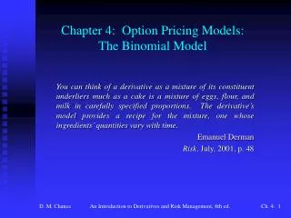
Chapter 4: Option Pricing Models: The Binomial Model
This chapter delves into the Binomial Model for option pricing, providing a comprehensive overview of essential concepts such as one-period and two-period models, risk-free hedging, and the implications of early exercise. It defines an option pricing model as a mathematical representation predicting an option’s fair value based on underlying factors. Through illustrative examples, this chapter explains how to create a hedged portfolio, evaluate European call options, and demonstrates the effects of price changes on returns. Key insights into alternative specifications and extensions of the binomial model are also discussed.

Chapter 4: Option Pricing Models: The Binomial Model
E N D
Presentation Transcript
Chapter 4: Option Pricing Models:The Binomial Model You can think of a derivative as a mixture of its constituent underliers much as a cake is a mixture of eggs, flour, and milk in carefully specified proportions. The derivative’s model provides a recipe for the mixture, one whose ingredients’ quantities vary with time. Emanuel Derman Risk, July, 2001, p. 48 An Introduction to Derivatives and Risk Management, 6th ed.
Important Concepts in Chapter 4 • The concept of an option pricing model • The one- and two-period binomial option pricing models • Explanation of the establishment and maintenance of a risk-free hedge • Illustration of how early exercise can be captured • The extension of the binomial model to any number of time periods • Alternative specifications of the binomial model An Introduction to Derivatives and Risk Management, 6th ed.
Definition of a model • A simplified representation of reality that uses certain inputs to produce an output or result • Definition of an option pricing model • A mathematical formula that uses the factors that determine an option’s price as inputs to produce the theoretical fair value of an option. An Introduction to Derivatives and Risk Management, 6th ed.
The One-Period Binomial Model • Conditions and assumptions • One period, two outcomes (states) • S = current stock price • u = 1 + return if stock goes up • d = 1 + return if stock goes down • r = risk-free rate • Value of European call at expiration one period later • Cu = Max(0,Su - X) or • Cd = Max(0,Sd - X) • See Figure 4.1, p. 98 An Introduction to Derivatives and Risk Management, 6th ed.
The One-Period Binomial Model (continued) • Important point: d < 1 + r < u to prevent arbitrage • We construct a hedge portfolio of h shares of stock and one short call. Current value of portfolio: • V = hS - C • At expiration the hedge portfolio will be worth • Vu = hSu - Cu • Vd = hSd - Cd • If we are hedged, these must be equal. Setting Vu = Vd and solving for h gives An Introduction to Derivatives and Risk Management, 6th ed.
The One-Period Binomial Model (continued) • These values are all known so h is easily computed • Since the portfolio is riskless, it should earn the risk-free rate. Thus • V(1+r) = Vu (or Vd) • Substituting for V and Vu • (hS - C)(1+r) = hSu - Cu • And the theoretical value of the option is An Introduction to Derivatives and Risk Management, 6th ed.
The One-Period Binomial Model (continued) • This is the theoretical value of the call as determined by the stock price, exercise price, risk-free rate, and up and down factors. • The probabilities of the up and down moves were never specified. They are irrelevant to the option price. An Introduction to Derivatives and Risk Management, 6th ed.
The One-Period Binomial Model (continued) • An Illustrative Example • S = 100, X = 100, u = 1.25, d = 0.80, r = .07 • First find the values of Cu, Cd, h, and p: • Cu = Max(0,100(1.25) - 100) = Max(0,125 - 100) = 25 • Cd = Max(0,100(.80) - 100) = Max(0,80 - 100) = 0 • h = (25 - 0)/(125 - 80) = .556 • p = (1.07 - 0.80)/(1.25 - 0.80) = .6 • Then insert into the formula for C: An Introduction to Derivatives and Risk Management, 6th ed.
The One-Period Binomial Model (continued) • A Hedged Portfolio • Short 1,000 calls and long 1000h = 1000(.556) = 556 shares. See Figure 4.2, p. 101. • Value of investment: V = 556($100) - 1,000($14.02) = $41,580. (This is how much money you must put up.) • Stock goes to $125 • Value of investment = 556($125) - 1,000($25) = $44,500 • Stock goes to $80 • Value of investment = 556($80) - 1,000($0) = $44,480 An Introduction to Derivatives and Risk Management, 6th ed.
The One-Period Binomial Model (continued) You invested $41,580 and got back $44,500, a 7 % return, which is the risk-free rate. • An Overpriced Call • Let the call be selling for $15.00 • Your amount invested is 556($100) - 1,000($15.00) = $40,600 • You will still end up with $44,500, which is a 9.6% return. • Everyone will take advantage of this, forcing the call price to fall to $14.02 An Introduction to Derivatives and Risk Management, 6th ed.
The One-Period Binomial Model (continued) • An Underpriced Call • Let the call be priced at $13 • Sell short 556 shares at $100 and buy 1,000 calls at $13. This will generate a cash inflow of $42,600. • At expiration, you will end up paying out $44,500. • This is like a loan in which you borrowed $42,600 and paid back $44,500, a rate of 4.46%, which beats the risk-free borrowing rate. An Introduction to Derivatives and Risk Management, 6th ed.
The Two-Period Binomial Model • We now let the stock go up another period so that it ends up Su2, Sud or Sd2. • See Figure 4.3, p. 105. • The option expires after two periods with three possible values: An Introduction to Derivatives and Risk Management, 6th ed.
The Two-Period Binomial Model (continued) • After one period the call will have one period to go before expiration. Thus, it will worth either of the following two values • The price of the call today will be An Introduction to Derivatives and Risk Management, 6th ed.
The Two-Period Binomial Model (continued) • The hedge ratios are different in the different states: An Introduction to Derivatives and Risk Management, 6th ed.
The Two-Period Binomial Model (continued) • An Illustrative Example • Su2 = 100(1.25)2 = 156.25 • Sud = 100(1.25)(.80) = 100 • Sd2 = 100(.80)2 = 64 • The call option prices are as follows An Introduction to Derivatives and Risk Management, 6th ed.
The Two-Period Binomial Model (continued) • The two values of the call at the end of the first period are An Introduction to Derivatives and Risk Management, 6th ed.
The Two-Period Binomial Model (continued) • Therefore, the value of the call today is An Introduction to Derivatives and Risk Management, 6th ed.
The Two-Period Binomial Model (continued) • A Hedge Portfolio • See Figure 4.4, p 109. • Call trades at its theoretical value of $17.69. • Hedge ratio today: h = (31.54 - 0.0)/(125 - 80) = .701 • So • Buy 701 shares at $100 for $70,100 • Sell 1,000 calls at $17.69 for $17,690 • Net investment: $52,410 An Introduction to Derivatives and Risk Management, 6th ed.
The Two-Period Binomial Model (continued) • A Hedge Portfolio (continued) • Note each of the possibilities: • Stock goes to 125, then 156.25 • Stock goes to 125, then to 100 • Stock goes to 80, then to 100 • Stock goes to 80, then to 64 • In each case, you wealth grows by 7% at the end of the first period. You then revise the mix of stock and calls by either buying or selling shares or options. Funds realized from selling are invested at 7% and funds necessary for buying are borrowed at 7%. An Introduction to Derivatives and Risk Management, 6th ed.
The Two-Period Binomial Model (continued) • A Hedge Portfolio (continued) • Your wealth then grows by 7% from the end of the first period to the end of the second. • Conclusion: If the option is correctly priced and you maintain the appropriate mix of shares and calls as indicated by the hedge ratio, you earn a risk-free return over both periods. An Introduction to Derivatives and Risk Management, 6th ed.
The Two-Period Binomial Model (continued) • A Mispriced Call in the Two-Period World • If the call is underpriced, you buy it and short the stock, maintaining the correct hedge over both periods. You end up borrowing at less than the risk-free rate. • If the call is overpriced, you sell it and buy the stock, maintaining the correct hedge over both periods. You end up lending at more than the risk-free rate. • See Table 4.1, p. 111 for summary. An Introduction to Derivatives and Risk Management, 6th ed.
Extensions of the Binomial Model • Pricing Put Options • Same procedure as calls but use put payoff formula at expiration. In our example the put prices at expiration are An Introduction to Derivatives and Risk Management, 6th ed.
Extensions of the Binomial Model (continued) • Pricing Put Options (continued) • The two values of the put at the end of the first period are An Introduction to Derivatives and Risk Management, 6th ed.
Extensions of the Binomial Model (continued) • Pricing Put Options (continued) • Therefore, the value of the put today is An Introduction to Derivatives and Risk Management, 6th ed.
Extensions of the Binomial Model (continued) • Pricing Put Options (continued) • Let us hedge a long position in stock by purchasing puts. The hedge ratio formula is the same except that we ignore the negative sign: • Thus, we shall buy 299 shares and 1,000 puts. This will cost $29,900 (299 x $100) + $5,030 (1,000 x $5.03) for a total of $34,930. An Introduction to Derivatives and Risk Management, 6th ed.
Extensions of the Binomial Model (continued) • Pricing Put Options (continued) • Stock goes from 100 to 125. We now have • 299 shares at $125 + 1,000 puts at $0.0 = $37,375 • This is a 7% gain over $34,930. The new hedge ratio is • So sell 299 shares, receiving 299($125) = $37,375, which is invested in risk-free bonds. An Introduction to Derivatives and Risk Management, 6th ed.
Extensions of the Binomial Model (continued) • Pricing Put Options (continued) • Stock goes from 100 to 80. We now have • 299 shares at $80 + 1,000 puts at $13.46 = $37,380 • This is a 7% gain over $34,930. The new hedge ratio is • So buy 701 shares, paying 701($80) = $56,080, by borrowing at the risk-free rate. An Introduction to Derivatives and Risk Management, 6th ed.
Extensions of the Binomial Model (continued) • Pricing Put Options (continued) • Stock goes from 125 to 156.25. We now have • Bond worth $37,375(1.07) = $39,991 • This is a 7% gain. • Stock goes from 125 to 100. We now have • Bond worth $37,375(1.07) = $39,991 • This is a 7% gain. An Introduction to Derivatives and Risk Management, 6th ed.
Extensions of the Binomial Model (continued) • Pricing Put Options (continued) • Stock goes from 80 to 100. We now have • 1,000 shares worth $100 each, 1,000 puts worth $0 each, plus a loan in which we owe $56,080(1.07) = $60,006 for a total of $39,994, a 7% gain • Stock goes from 80 to 64. We now have • 1,000 shares worth $64 each, 1,000 puts worth $36 each, plus a loan in which we owe $56,080(1.07) = $60,006 for a total of $39,994, a 7% gain An Introduction to Derivatives and Risk Management, 6th ed.
Extensions of the Binomial Model (continued) • American Puts and Early Exercise • Now we must consider the possibility of exercising the put early. At time 1 the European put values were • Pu = 0.00 when the stock is at 125 • Pd = 13.46 when the stock is at 80 • When the stock is at 80, the put is in-the-money by $20 so exercise it early. Replace Pu = 13.46 with Pu = 20. The value of the put today is higher at An Introduction to Derivatives and Risk Management, 6th ed.
Extensions of the Binomial Model (continued) • Dividends, European Calls, American Calls, and Early Exercise • One way to incorporate dividends is to assume a constant yield, , per period. The stock moves up, then drops by the rate . • See Figure 4.5, p. 114 for example with a 10% yield • The call prices at expiration are An Introduction to Derivatives and Risk Management, 6th ed.
Extensions of the Binomial Model (continued) • Dividends, European Calls, American Calls, and Early Exercise (continued) • The European call prices after one period are • The European call value at time 0 is An Introduction to Derivatives and Risk Management, 6th ed.
Extensions of the Binomial Model (continued) • Dividends, European Calls, American Calls, and Early Exercise (continued) • If the call is American, when the stock is at 125, it pays a dividend of $12.50 and then falls to $112.50. We can exercise it, paying $100, and receive a stock worth $125. The stock goes ex-dividend, falling to $112.50 but we get the $12.50 dividend. So at that point, the option is worth $25. We replace the binomial value of Cu = $22.78 with Cu = $25. At time 0 the value is An Introduction to Derivatives and Risk Management, 6th ed.
Extensions of the Binomial Model (continued) • Dividends, European Calls, American Calls, and Early Exercise (continued) • Alternatively, we can specify that the stock pays a specific dollar dividend at time 1. Assume $12. Unfortunately, the tree no longer recombines, as in Figure 4.6, p. 115. We can still calculate the option value but the tree grows large very fast. See Figure 4.7, p. 116. • Because of the reduction in the number of computations, trees that recombine are preferred over trees that do not recombine. An Introduction to Derivatives and Risk Management, 6th ed.
Extensions of the Binomial Model (continued) • Dividends, European Calls, American Calls, and Early Exercise (continued) • Yet another alternative (and preferred) specification is to subtract the present value of the dividends from the stock price (as we did in Chapter 3) and let the adjusted stock price follow the binomial up and down factors. For this problem, see Figure 4.8, p. 117. • The tree now recombines and we can easily calculate the option values following the same procedure as before. An Introduction to Derivatives and Risk Management, 6th ed.
Extensions of the Binomial Model (continued) • Dividends, European Calls, American Calls, and Early Exercise (continued) • The option prices at expiration are An Introduction to Derivatives and Risk Management, 6th ed.
Extensions of the Binomial Model (continued) • Dividends, European Calls, American Calls, and Early Exercise (continued) • At time 1 the option prices are • We exercise at time 1 so that Cu is now 22.99. At time 0 • The European option value would be 12.18. An Introduction to Derivatives and Risk Management, 6th ed.
Extensions of the Binomial Model (continued) • Extending the Binomial Model to n Periods • With n periods to go, the binomial model can be easily extended. There is a long and somewhat complex looking formula in the book. The basic procedure, however, is the same. See Figure 4.9, p. 119 in which we see below the stock prices the prices of European and American puts. This illustrates the early exercise possibilities for American puts, which can occur in multiple time periods. • At each step, we must check for early exercise by comparing the value if exercised to the value if not exercised and use the higher value of the two. An Introduction to Derivatives and Risk Management, 6th ed.
Extensions of the Binomial Model (continued) • The Behavior of the Binomial Model for Large n and a Fixed Option Life • The risk-free rate is adjusted to (1 + r)T/n • The up and down parameters are adjusted to • where is the volatility. Let us price the AOL June 125 call with one period. An Introduction to Derivatives and Risk Management, 6th ed.
Extensions of the Binomial Model (continued) • The Behavior of the Binomial Model for Large n and a Fixed Option Life (continued) • The parameters are now • The new stock prices are • Su = 125.9375(1.293087) = 162.8481 • Sd = 125.9375(0.773343) = 97.3929 An Introduction to Derivatives and Risk Management, 6th ed.
Extensions of the Binomial Model (continued) • The Behavior of the Binomial Model for Large n and a Fixed Option Life (continued) • The new option prices would be • Cu = Max(0,162.8481-125) = 37.85 • Cd = Max(0,97.3929 - 125) = 0.0 • p would be (1.004285 - 0.773343)/(1.293087 - 0.773343) = .444; 1 - p = .556. • The price of the option at time 0 is, therefore, An Introduction to Derivatives and Risk Management, 6th ed.
Extensions of the Binomial Model (continued) • The Behavior of the Binomial Model for Large n and a Fixed Option Life (continued) • The actual price of the option is 13.50, but obviously one binomial period is not enough. • Table 4.2, p. 121 shows what happens as we increase the number of binomial periods. The price converges to around 13.56. In Chapter 5, we shall see that this is approximately the Black-Scholes price. An Introduction to Derivatives and Risk Management, 6th ed.
Extensions of the Binomial Model • Alternative Specifications of the Binomial Model • We can use a different specification of u, d and p • where ln(1 + r) is the continuously compounded interest rate. Here p will converge to .5 as n increases. An Introduction to Derivatives and Risk Management, 6th ed.
Extensions of the Binomial Model • Alternative Specifications of the Binomial Model (continued) • Now let us price the AOL June 125 call but use two periods. We have r = (1.0456)0.0959/2 - 1 = .0021. Using our previous formulas, An Introduction to Derivatives and Risk Management, 6th ed.
Extensions of the Binomial Model • Alternative Specifications of the Binomial Model (continued) • Now let us use these new formulas: • We can use .5 for p. See Figure 4.10, p. 123. The prices are close and will converge when n is large. • See bsbin3.xls and bsbwin2.2 for software to calculate the binomial model. An Introduction to Derivatives and Risk Management, 6th ed.
Summary An Introduction to Derivatives and Risk Management, 6th ed.
(Return to text slide) An Introduction to Derivatives and Risk Management, 6th ed.
(Return to text slide) An Introduction to Derivatives and Risk Management, 6th ed.
(Return to text slide) An Introduction to Derivatives and Risk Management, 6th ed.
(Return to text slide) An Introduction to Derivatives and Risk Management, 6th ed.