Download
1 / 24
240 likes | 495 Vues
THEORY OF CONSTRAINTS. 1998. 2. 28 송 태 영. REFERENCES. Computerized shop floor scheduling. 1988. IJPR Optimum Production Technology & the Theory Of Constraints : analysis and genealogy. 1995. IJPR

E N D
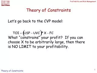
THEORY OF CONSTRAINTS 1998. 2. 28 송 태 영
REFERENCES • Computerized shop floor scheduling. 1988. IJPR • Optimum Production Technology & the Theory Of Constraints : analysis and genealogy. 1995. IJPR • Comparing JIT, MRP, and TOC, and embedding TOC into MRP. 1997. IJPR • ELIYAHU M. GOLDRATT* • M. S. SPENCER and J. F. COX** • J.MILTENBURG*** • * Avraham Y. Goldratt Institute • ** Dep of management, College of Business Administration, Univ of Northern Iowa • *** Dep of Management, The Terry College of business, Univ of Georgia
INTRODUCTION • 1.OPT에서 TOC까지 :TOC의 계보 • 2. The elements comprise TOC • 3. Embedding TOC into MRP • 4. Case study
CONFUSION • differences between OPT & TOC • elements that comprise the twomethods • ‘the goal’ presents practical concept - is it for OPT or TOC?
1. OPT에서 TOC까지 • Identifying time frame of methods • OPT(1979)Optimized Production Timetables computerized scheduling, thoughtware was in its infancy • OPT(1980s)technology broaden it’s application from shop floor scheduling to jobshop environment with halt concept (cf. stop) • ‘The goal’(1984) • version 56 OPT s/w(1985~1986) • there was no BM, DBR methodology • OPT should be limited to s/w concept ; provides finite scheduling methodology based on max of production though bottleneck operation. There was no solidified DBR elements, measurement system, thoughtware.
‘The Goal’ provides 5 step for DBR concepts • 1. Identifying the constraints • 2.deciding how to exploit the constraint • 3.subordinating all other activities to the constraint • 4.elevating the constraint • 5.continuous improvement step of admonishing against managerial inertia • Buffer Management; predict potential shortage, trigger preventative action(ex.), focus for continuous improvement process for shop operations. • In conclusion ‘the goal’ suggests Scheduling process -> exploring the underlying concepts
Theory of Constraints Logistics Problem solving/ thinking process ECE diagrams Cloud diagrams Five-Step focusing process Scheduling process V-A-T analysis ECE audit Five-Step focusing process DBR Buffer management Performance system Throughput Inventory Operating expense Product mix Throughput dollar days Inventory dollar days 2. The elements comprise TOC • Underlying concepts drew increased attention. • TOC(1987 ~ 1993) significant ramification - accounting, marketing, product design
Most visibility to operation manager V-A-T: identify the positioning of the buffer based on combination of the BOM structure & components, assembly routeings Logistics Logistics Five-Step focusing Scheduling process V-A-T analysis DBR Buffer management
Performance system • Developed in ‘The goal’ to support the management of constraint & eliminate the conflict with traditional performance measurement • The throughput-dollar-days measurement facilitates operating decision that support goal of firm to increase net profit return on investment with a positive cash flow Performance system Throughput Inventory Operating expense Product mix Throughput dollar days Inventory dollar days
Problem solving/ thinking process • The least researched and least visible branch to operation managers • efficiency~innovation in IE • focuses on resolving what to change, to change what, how to bring about change • ECE diagram • ECE audit process • cloud diagram Problem solving/ thinking process ECE diagrams Cloud diagrams ECE audit Five-Step focusing process
3. Embedding TOC into MRP • MRP, JIT, TOC • MRP is so flexible that it can behave like JIT,TOC • Five-step technical procedure with an ex. • Spencer(1991): MRP rough cut plan is used to identify the bottleneck resource. Then a schedule is developed and create MPS for all end product. Buffer at shipping, assemble, bottleneck.
5 Step IN LOGICS • Step1: Determine the constraints. • Step2: Set time buffers, revise routeings and leadtime • Step3: Set drum schedule, compute MPS • Step4: Use MRP algebra to schedule workcenters • Step5: Control production, measure performance
Step1: Determine the constraints • n = # of product m = # of workcenters i = index for a product(i=1,…,n) j = index for a workcenters(j = 1,…,m) Di = planned demand for product i noi = # of operations required to produce product i ki = kth operation on product i (ki = 1,…,noi) w(i, ki) = workcenter where operation ki is performed p(I, ki) = processing time for operation ki • Lj = at workcenter j • LP is the tool for the most profitable manner • If no constraint, market is the one.
Step2: Set time buffers, revise routeings and leadtime • Time buffers are set (up, downstream) • It becomes phantom workcenter set up in MRP • processing time = time to set up and complete processing of one process batch (the same as MRP)
Step3: Set drum schedule, compute MPS • Scheduling and production control follow ‘drum - buffer - rope’ • drum: developed schedule that most profitably max utilization at the constraint • schedule -> MPS through rope -> MRP algebra(order releases, due date, schedule for all workcenters)
Step4: Use MRP algebra to schedule workcenters • Workcenter must complete their order on time • TOC uses 2 procedures for ensure this • non-constraint workcener produce orders as soon as they arrives • buffer management is used - buffer is monitored, if it gets low production is expedited • w* = constraint workcenter I* = size of time buffer r(i,1) = readytime or release date of product i to the workcenter performing the first operation Qi = # of units in a process batch of product i. T(i,ki) = tie to complete processing of operation ki for one process batch of product i. d(i,ki) = due date for completion of operation ki. si = promised shopping date for product i. LTi = manufacturing lead time for product i. • Then d(i,ki) = d(i, ki - 1) + t(i, ki) i = 1,…,n; ki = 1,…,noi d(i,0) = r(i,1) LTi = d(i, noi) - r(i,1) • In make - to - stock, make - to - order • when products have the same due dates, products with higher value-added are produced
Step5: Control production, measure performance • performance is measured by comparing actual production with scheduled production • not earlyand not late • achieving by penalizing • S(w,t) = Scheduled at workcenter w for time period t to t + 1. c(i, ki) = Actual completion date of operation ki for product i. Vi = dollar value of one process batch of product i after all oprations are completed. he = penalty per time period per unit of value for completing production early. ht = penalty per time period per unit of value for completing production late. M(w,t) = 100%[1 - (M’(w,t)/M”(w,t))] where • M’(w,t)= (Vi/noi)*max[he(d(i,ki) - c(i,ki)), ht(c(i,ki) - d(i,ki))] • M”(w,t)= (Vi/noi) • The smaller M(w,t)is, the poor as the actual production compared the scheduled one
Case:Microelectronics plant • The IC’s are produced on wafers on average of 28 operations, completed over a cycle time of 41 days at 15 workcenters • Figure 2 Product and demand
Determine the constraint compute the planned load Lj PHOT is the constraint (126 = 5.25 * 10 + 4.5 * 7 + 5.25*7) figure 3 work center capacities and loads STEP1
STEP2 • Setting buffer • prevention stoppage at the constraints • size of buffer is one day of PHOT(It depends) • If products from PHOT merge with products there should be one more buffer • As a result • total time 28 days Mfg lead time 28 days
Set the drum schedule, compute MPS at A,B,C the Portion of demand that will be satisfied is determined by LP product mix A = 4 B = 4 C = 5 notice that Prod_A has a higher profit margin than Prod_B Because A,B,C are make - to- stock the drum schedule & MPS can be balanced Mon ~ Thurday C, B, A Friday C Max 4000X1+3000X2+4200X3 st. 70X1+49X2+56X6 < 770 X1 < 5.25 X2 < 4.5 X3 < 5.25 STEP 3
STEP4 • Use MRP algebra to schedule work center • process batch is 24wafers but transfer batch varies • orders are released to the plant according to balanced schedule in step 3 • released date r(i,1), due date d(i,ki), for all prod at all work center are computed from equation 2. • Figure 4. Calculation ready times and due dates
STEP 5 • Control production, measure performance • dispatch list at all work center including buffers • work center performance from equation 4. • Ex. OX4 work center
CONCLUSION • TOC is also useful tool for accounting, marketing and product design • Comparing JIT & TOC • TOC needs some inventory while JIT tries to eliminates it • TOC provides tool for solving problems • elevating constraints, buffer management, improvement activities are more focused