Statistics for Microarrays
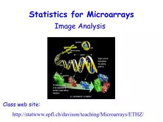
Statistics for Microarrays. Image Analysis. Class web site: http://statwww.epfl.ch/davison/teaching/Microarrays/ETHZ/. Biological question Differentially expressed genes Sample class prediction etc. Experimental design. Microarray experiment. 16-bit TIFF files. Image analysis.

Statistics for Microarrays
E N D
Presentation Transcript
Statistics for Microarrays Image Analysis Class web site: http://statwww.epfl.ch/davison/teaching/Microarrays/ETHZ/
Biological question Differentially expressed genes Sample class prediction etc. Experimental design Microarray experiment 16-bit TIFF files Image analysis (Rfg, Rbg), (Gfg, Gbg) Normalization R, G Estimation Testing Clustering Discrimination Biological verification and interpretation
Scanner PMT Pinhole Detector lens Laser Beam-splitter Objective Lens Dye Glass Slide
Scanner Process A/D Convertor Laser PMT Dye Electrons Signal Photons excitation amplification Filtering Time-space averaging
Quantification of Expression For each spot on the slide, calculate Red intensity = Rfg - Rbg (fg = foreground, bg = background) and Green intensity = Gfg - Gbg and combine them in the log (base 2) ratio Log2(Red/Green)
Practical Problems 1 Comet Tails • Likely caused by insufficiently rapid immersion of the slides in the succinic anhydride blocking solution
Practical Problems 2 Blotches, unequal spot sizes, overlapping spots
Practical Problems 3 High Background • 2 likely causes: • Insufficient blocking • Precipitation of the labeled probe Weak Signals
Practical Problems 4 • Spot overlap • Likely cause: Too much rehydration • during post - • processing.
Practical Problems 5 Dust
Images from scanner • Resolution • standard 10m [currently, max 5m] • 100m spot on chip = 10 pixels in diameter • Image format • TIFF (tagged image file format) 16 bit (65,536 levels of gray) • 1cm x 1cm image at 16 bit = 2Mb (uncompressed) • other formats exist e.g. SCN (used at Stanford) • Separate image for each fluorescent sample • channel 1, channel 2, etc.
Images in analysis software • The two 16-bit images (Cy3, Cy5) are compressed into 8-bit images • Display fluorescence intensities for both wavelengths using a 24-bit RGB overlay image • RGB image : • Blue values (B) are set to 0 • Red values (R) are used for Cy5 intensities • Green values (G) are used for Cy3 intensities • Qualitative representation of results
Pseudo-color overlay Cy3 Cy5 Images : examples
Steps in Images Processing • Addressing (or Gridding) • Assigning coordinates to each spot • Segmentation • Classification of pixels as either foreground (signal) or background • Information Extraction • Foreground fluorescence intensity pairs (R, G) • Background intensities • Quality measures
Addressing This is the process of assigning coordinates to each of the spots. Automating this part of the procedure permits high throughput analysis. 4 by 4 grids 19 by 21 spots per grid
Addressing Within the same batch of print runs; estimate translation of grids Other problems: — Misregistration — Rotation — Skew in the array 4 by 4 grids
Problems in automatic addressing Misregistration of the red and green channels Rotation of the array in the image Skew in the array Rotation
ScanAlyze Addressing (I) • Basic structure of images known (determined by the arrayer) • Parameters to address spot positions • Separation between rows and columns of grids • Individual translation of grids • Separation between rows and columns of spots within each grid • Small individual translation of spots • Overall position of the array in the image
Addressing (II) • The measurement process depends on the addressing procedure • Addressing accuracy can be enhanced by allowing user intervention (at the cost of time) • Most software systems now provide for both manual and automatic gridding procedures
Segmentation • Classification of pixels as foreground or background fluorescence intensities are calculated for each spot as measure of transcript abundance • Production of a spot mask : set of foreground pixels for each spot
Segmentation Methods • Fixed circles • Adaptive circles • Adaptive shape • Edge detection • Seeded Region Growing (R. Adams and L. Bishof (1994): Regions grow outwards from seed points preferentially according to the difference between a pixel’s value and the running mean of values in an adjoining region • Histogram methods
May not be goodfor this example Fixed circle segmentation • Fits a circle with a constant diameter to all spots in the image • Easy to implement • The spots should be of the same shape and size
Dapple finds spots by detecting edges of spots (second derivative) Adaptive circle segmentation • The circle diameter is estimated separately for each spot • Problematic if spot exhibits oval shapes
Limitation of circular segmentation • Small spot • Not circular Results from SRG
Limitation of fixed circles SRG Fixed Circle
Adaptive shape segmentation • Specification of starting points or seeds • Bonus: already know geometry of array • Regions grow outwards from the seed points preferentially according to the difference between a pixel’s value and the running mean of values in an adjoining region
Bkgd Foreground Histogram segmentation • Choose target mask larger than any spot • Fg and bg intensities determined from the histogram of pixel values for pixels within the masked area • Example : QuantArray • Background : mean between 5th and 20th percentile • Foreground : mean between 80th and 95th percentile • May not work well when a large target mask is set to compensate for variation in spot size
Information Extraction • Spot Intensities • mean of pixel intensities • median of pixel intensities • Pixel variation (e.g. IQR) • Background values • None • Local • Constant (global) • Morphological opening • Quality Information Take the average
Background intensity • The measured fluorescence intensity includes a contribution of non-specific hybridization and other chemicals on the glass • Fluorescence from regions not occupied by DNA should be different from regions occupied by DNA one solution is to use local negative controls (spotted DNA that should not hybridize)
BG: None • Do not consider the background • Probably not accurate in many cases, but may be better than some forms of local background determination
ScanAlyze ImaGene Spot, GenePix BG: Local • Focusing on small regions surrounding the spot mask • Median of pixel values in this region • Most software package implement such an approach • By not considering the pixels immediately surrounding the spots, the background estimate is less sensitive to the performance of the segmentation procedure
BG: Constant • Global method which subtracts a constant background for all spots • Some evidence that the binding of fluorescent dyes to ‘negative control spots’ is lower than the binding to the glass slide • More meaningful to estimate background based on a set of negative control spots • If no negative control spots :approximation of the average background =third percentile of all the spot foreground values
BG: Morphological opening • Non-linear filtering, used in Spot • Use a square structuring element with side length at least twice as large as the spot separation distance • Compute local minimum filter, then compute local maximum filter • This removes all spots and generates an image that is an estimate of the background for the entire slide • For individual spots, the background is estimated by sampling this background image at the nominal center of the spot • Lower, less variable bg estimate
Background matters From Spot From GenePix
Quality Measurements • Array • Correlation between spot intensities • Percentage of spots with no signals • Distribution of spot signal area • Spot • Signal / Noise ratio • Variation in pixel intensities • Identification of “bad spot” (spots with no signal) • Ratio (2 spots combined) • Circularity • Flag or weight spots based on these (or other appropriate) criteria
Quality of Array • Distribution of areas • - Judge by eye • - Look at variation. (e.g. SD) • Cy3 area • mean 57 • median 56 • SD 20.67 • Cy5 area • mean 59 • median 57 • SD 24.34
M = log2 R/G A = log2 √(R•G) Spot, GenePix ScanAlyze Summary • The choice of background correction method often has a larger impact on the log-intensity ratios than the segmentation method used • The morphological opening method provides a better estimate of background than other methods • Low within- and between-slide variability of the log2 R/G • Background adjustment has a larger impact on low intensity spots
Selected references • Yang, Y. H., Buckley, M. J., Dudoit, S. and Speed, T. P. (2001), ‘Comparisons of methods for image analysis on cDNA microarray data’. Technical report #584, Department of Statistics, University of California, Berkeley.http://www.stat.berkeley.edu/users/terry/zarray/Html/papersindex.html • Yang, Y. H., Buckley, M. J. and Speed, T. P. (2001), ‘Analysis of cDNA microarray images’. Briefings in bioinformatics, 2 (4), 341-349.Excellent review in concise format!
Terry Speed Michael Buckley Sandrine Dudoit Natalie Roberts Ben Bolstad Brian Stevenson CSIRO Image Analysis Group Ryan Lagerstorm Richard Beare Hugues Talbot Kevin Cheong Matt Callow (LBL) Percy Luu (USB) Dave Lin (USB) Vivian Pang (USB) Elva Diaz (USB) Acknowledgments