Atmospheric Radiation: Clouds Parameterization
Explore atmospheric radiation and cloud structure quantification, the impact of sub-grid cloud structure, and 3D radiative transport. Discover the radiative impact and efficiency of representing cloud structures.

Atmospheric Radiation: Clouds Parameterization
E N D
Presentation Transcript
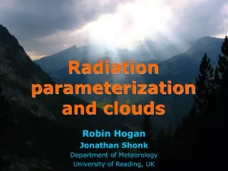
Radiation parameterization and clouds Robin Hogan Jonathan Shonk Department of Meteorology University of Reading, UK
Overview • From Maxwell to the two-stream approximation • Quantifying sub-grid cloud structure from observations • The challenge of representing cloud structure efficiently • What is the global radiative impact of sub-grid cloud structure? • Do we need to worry about 3D radiative transport? • Are we spending our computer time wisely? • Outlook
What does a radiation scheme do? The bit of the model that takes so long to run Radiation in the presence of clouds tends to destabilize the atmosphere Sn Ln • Variables on model grid • Temperature, pressure, humidity, ozone • Cloud liquid and ice mixing ratios • Cloud fraction
Building blocks of atmospheric radiation p E Oscillating dipole p is induced, which is typically in phase with the incident electric field E Dipole radiates in all directions (except directly parallel to its axis) • Emission and absorption of quanta of radiative energy • Governed by quantum mechanics: the Planck function and the internal energy levels of the material • Responsible for complex gaseous absorption spectra • Electromagnetic waves interacting with a dielectric material • An oscillating dipole is excited, which then re-radiates • Governed by Maxwell’s equations + Newton’s 2nd law for bound charges • Responsible for scattering, reflection and refraction + −
Maxwell’s equations • Almost all atmospheric radiative phenomena are due to this effect, described by the Maxwell curl equations: • where c is the speed of light in vacuum, n is the complex refractive index (which varies with position), and E and B are the electric and magnetic fields (both functions of time and position); • It is illuminating to discretize these equations directly • This is known as the Finite-Difference Time-Domain (FDTD) method • Use a staggered grid in time and space (Yee 1966) • Consider two dimensions only for simplicity • Need gridsize of ~0.02 mm and timestep of ~50 ps for atmospheric problems By Ez Ez Bx Bx By Ez Ez
Simple examples • Refraction (a mirage) • Rayleigh scattering (blue sky) n gradient Single dipole Scattered field (total − incident) Refractive index Total Ez field
More complex examples • A sphere (or circle in 2D) • An ice column Scattered field (total − incident) Refractive index Total Ez field Many more animations at www.met.rdg.ac.uk/~swrhgnrj/maxwell (interferometer, diffraction grating, dish antenna, clear-air radar…)
The phase function q • The distribution of scattered energy is known as the “scattering phase function” • Different methods are suitable for different types of scatterer • Spheres: Mie theory (Mie 1908) provides a solution to Maxwell’s equations as a series expansion • Arbitrary ice particle shapes: depending on D/l, use the Discrete Dipole Approximation, FDFT or ray tracing (Yang et al. 2000) • But observations (Baran) suggest smoother phase functions implying that the surface of ice particles is “rough”
From Maxwell to radiative transfer Mishchenko et al. (2007) Maxwell’s equations in terms of fields E(x,t), B(x,t) Reasonable assumptions: • Ignore polarization • Ignore time-dependence (sun is a continuous source) • Particles are randomly separated so intensities add incoherently and phase is ignored • Random orientation of particles so phase function doesn’t depend on absolute orientation • No diffraction around features larger than individual particles 3D radiative transfer in terms of radiances I(x,W,n) in W m-2 sr-1 Hz-1
The 3D radiative transfer equation Loss by absorption or scattering Source Such as thermal emission Gain by scattering Radiation scattered from all other directions • Also known as the “Boltzmann transport equation”, this describes the radiance I in direction W (where the x and n dependence of all variables is implicit): • This may be solved in a 3D domain • Monte Carlo method most efficient for fluxes • As a boundary-value problem (e.g. using “SHDOM”) for radiances • Extinction coefficient be (m-1) is a key variable • When particle size >> wavelength, GCM can use Spatial derivative representing how much radiation is upstream
Two-stream approximation 3D radiative transfer in terms of radiances I(x,W,n) Unreasonable assumptions: • Radiances in all directions represented by only 2 (or sometimes 4) discrete directions • Atmosphere within a model gridbox is horizontally infinite and homogeneous • Details of the phase functions represented by one number, the asymmetry factor 1D radiative transfer in terms of two fluxes F(z,n) in W m-2 Hz-1
Discretized two-stream scheme Source terms S+, S Shortwave: scattering of direct solar beam Longwave: thermal emission • Equations relating diffuse fluxes between levels take the form: • Terms T, R and S given by Meador and Weaver (1980) Diffuse TOA sourceS0 F0.5+ F0.5 Reflection R, TransmissionT Layer 1 F1.5+ F1.5 Layer 2 F2.5+ F2.5 Surface sourceSs+,albedoas
Solution for two-level atmosphere • Solve the following tri-diagonal system of equations • Efficient to solve and simple to extend to more layers • But need to account for scattering and absorption by gases and clouds • Next we compare the problems posed by each
Gases • Gas absorption and scattering: • Varies with frequency n but not much with horizontal position x • Strongly vertically correlated • Well known spectrum for all major atmospheric gases • No significant transfer between frequencies (except Raman - tiny) • Correlated-k-distribution method for gaseous absorption • ECMWF (RRTM): 30 bands with a total of 252 independent calculations • Met Office (HadGEM): 15 bands with 130 independent calculations
Clouds • Cloud absorption and scattering: • Varies with horizontal position xand (somewhat less) with frequency n • Not very vertically correlated • Exact distribution within model gridbox is unknown • Horizontal transfer can be significant • Independent column approximation (ICA) • Divide atmosphere into non-interacting horizontally-infinite columns • Need ~50 columns implying ~104 independent calculations with gases • Too computationally expensive for a large-scale model! Radar-lidar retrievals and radiation observations from Lindenberg, 19 April 2006
Many issues to resolve • Model cloud scheme provides cloud fraction and water content but not cloud structure information • Some newer schemes prognose cloud variability (e.g. Tompkins 2002, Wilson et al. 2008) but they need validation • So we need the following from observations: • The degree to which clouds in different layers are overlapped • The horizontal variability of water content within a grid box • The degree to which cloud inhomogeneities are overlapped • But the independent column approximation is too expensive to use anyway • What tricks can we employ to represent cloud structure efficiently? • Is ICA OK or do we need to represent 3D effects as well? • What is the impact of these factors on radiation globally?
Cloud overlap assumption in models • Three possible overlap assumptions: • These assumptions generate very different cloud covers • Different radiative properties for same water content & cloud fraction • Most models still use “maximum-random” overlap but, how good is it?
Cloud radar sites A-Train of satellites • Key cloud instruments at each site: • Radar, lidar and microwave radiometers Chilbolton 35 GHz “Copernicus” radar
Cloud overlap from radar: example • Radar can observe the actual overlap of clouds • We next quantify the overlap from 3 months of data
Cloud overlap: approach • Consider combined cloud cover of pairs of levels • Group into vertically continuous and non-continuous pairs • Plot combined cloud cover versus level separation • Compare true cover & values from various overlap assumptions • Define overlap parameter a: 0 = random and 1 = maximum overlap
Cloud overlap: results • Vertically isolated clouds are randomly overlapped • Overlap of vertically continuous clouds becomes rapidly more random with increasing thickness, characterised by an overlap decorrelation length z0 ~ 1.6 km Hogan and Illingworth (QJ 2000)
“Exponential-random overlap” • Real atmosphere described by “exponential-random overlap” (or “decorrelation overlap”) • This is on average; overlap can be anything in individual cases • Need global observations to estimate z0 for different cloud types
Cloud overlap globally • CloudSat implies clouds are more maximally overlapped • But it also includes precipitation, which is more upright than clouds CloudSat (Mace) • Latitudinal dependence of z0 from ARM sites and Chilbolton • More convection and less shear in the tropics Maximum overlap P0 = 244.6 – 2.328 φ TWP (Mace & Benson 2002) SGP (Mace & Benson 2002) Chilbolton (Hogan & Illingworth 2000) NSA (Mace & Benson 2002) Random overlap
Further work required We should really define decorrelation length as a function of: • Liquid and ice; horizontal and vertical resolution • Malcolm Brooks (PhD 2005): ice more maximally overlapped than liquid: • But what is the global dependence, and what is the physics behind it? • Wind shear • Preliminary work suggests the dependence is weak • Convective versus stratiform clouds…
An interesting detail… • But most max-rand implementations give this: • Fluxes are usually homogenized in a cloudy or clear-sky region so have no memory of their horizontal distribution when entering another layer • Which one is right? B A If gridbox was slightly smaller, we see that A wrongly gives maximum overlap for non-adjacent layers, so B more correct. Good news: only adjacent-level overlap parameter is required! • Do we need to know the overlap of a layer with every other layer, or just with the adjacent layers? • We might expect “max-rand” overlap to give this: • Layer 1 is maximally overlapped with layer 3 because the cloud is “vertically continuous” 1 2 3
Why is cloud structure important? Clear air Cloud Inhomogeneous cloud • An example of non-linear averaging • Non-uniform clouds have lower mean emissivity & albedo for same mean optical depth due to curvature in the relationships Infrared absorption optical depth
Example from MODIS • By scaling the optical depth it appears we can get an unbiased fit to the true top-of-atmosphere albedo MODIS Stratocumulus 100-km boxes Plane-parallel albedo True mean albedo PP albedo for scaled optical depth Joe Daron and Itumeleng Kgololo
But satellites show optimum scaling factor is sensitive to Cloud type Gridbox size Solar zenith angle Shortwave/longwave Mean optical depth itself Also, better performance at top-of-atmosphere can mean worse performance in heating rate profile Need to measure variance of cloud properties and apply in a more sophisticated method Scaling factor from MODIS
Cirrus fallstreaks and wind shear Chilbolton 94-GHz cloud radar • Can estimate IWC from radar reflectivity and temperature • PDFs of IWC within can often be fitted by a lognormal distribution with a particular fractional variance: Low shear High shear Unified Model Hogan and Illingworth (JAS 2003) Hogan & Illingworth (2003)
18 months’ data • fIWC is the area under the power spectrum of ln(IWC) • Shear-induced mixing homogenises small scales • Scale break observed at ~50 km • Not sure why… Cloud top -5/3 Cloud base -3.5 Scale break ~50 km Gridbox size Hogan and Kew (QJ 2005) • Fractional variance increases with gridbox size d, decreases with wind shear s • log10fIWC = 0.3log10d - 0.04s - 0.93 • It becomes flat for d>50 km • Why? Shear-induced mixing at small scales
Observations of horizontal structure Rossow et al. (2002) Satellite (ISCCP) Cahalan et al. (1994) Microwave radiometer Shonk and Hogan (2008) Radar & microwave radiometer Sc Sc, Ac, Ci Ci Ci Cu Sc Ci Sc Sc & Ci Barker et al. (1996) Satellite (LandSat) Hogan and Illingworth (2003) Radar Smith and DelGenio (2001) Aircraft Oreopoulos and Cahalan (2005) Satellite (MODIS) • Typical fractional standard deviation ~0.75 Shonk (PhD, 2008)
Structure versus cloud fraction • For partially cloudy skies, cloud horizontal structure is not completely independent • Consider an underlying Gaussian distribution of total water • This results in fractional standard deviation tending to around unity for low cloud fractions • This is not inconsistent with LandSat observations
Overlap of inhomogeneities • For ice clouds, decorrelation length increases with gridbox size and decreases with shear Lower emissivity and albedo Higher emissivity and albedo Increasing shear • Radar retrievals much less reliable in liquid clouds • Many sub-grid models simply assume decorrelation length for cloud structure is half the decorrelation length for cloud boundaries • We now have the necessary information on cloud structure, but how can it be efficiently modelled in a radiation scheme?
Monte-Carlo ICA • McICA solves this problem • Each wavelength (and correlated-k quadrature point) receives a different profile -> only ~102 profiles • Modest amount of random noise not believed to affect forecasts GCM Observations Cloud fraction Water content (Variance?) Variance Overlap assumption • Generate random sub-columns of cloud • Statistics consistent with horizontal variance and overlap rules • ICA could be run on each • But double integral (space and wavelength) makes this too slow (~104 profiles) Cloud generator Raisanen et al. (2004) Water content Height Horizontal distance Pincus, Barker and Morcrette (2003)
Use Edwards-Slingo method as example Adapt two-stream method for two regions Matrix is now denser (pentadiagonal rather than tridiagonal) Traditional cloud fraction approach a b Layer 1 a b Layer 2 Note that coefficients describing the overlap between layers have been omitted
But some elements represent unwanted anomalous horizontal transport Remove them for a better solution But this is not enough… Anomalous horizontal transport a b Layer 1 Rab a b Layer 2 Rab is the reflection from region a to region b at the same level
Anomalous horizontal transport • Homogenization of clear-sky fluxes: • Reflected radiation has more chance to be absorbed -> TOA shortwave bias • Effect is very small in the longwave • This problem can be solved in a way that makes the code more efficient Cloud-fraction representation Independent column approximation
Solution Calculate upwelling and downwelling fluxes layer by layer At layer interfaces, use a weighted average of albedos according to overlap rules aa+1.5 aa-1.5 ab-1.5 Calculate albedo below level 1 for each region a2.5 New solver agrees very well with ICA Calculate albedo of entire atmosphere below level 2 • Anomalous horizontal transport almost entirely eliminated • Works in longwave and shortwave • Procedure is identical to Gaussian elimination and back-substitution in the case of 1 region • New solvers now available in Edwards-Slingo code • Easily extended to 3 or more regions Layer 1 Layer 2 Layer 3 Surface albedoas
How many regions are needed? • Lets try three regions first… • If the full PDF is known, use the 16th percentile for lower region • If we know only variance , then use p(LWC) • Continuous distribution • Four regions? • Three regions? • Two regions? • Standard plane-parallel approach LWC
Ice water content from Chilbolton, log10(kg m–3) Plane-parallel approx: 2 regions in each layer, one clear and one cloudy “Tripleclouds”: 3 regions in each layer Alternative to McICA Uses Edwards-Slingo capability for stratiform/convective regions for another purpose A new approach Height (km) Height (km) Height (km) Time (hours) Shonk and Hogan (JClim 2008)
Testing on 98 cloud radar scenes Tripleclouds: less than 1% bias and a smaller random error Plane-parallel assumption: 8% bias Scaling factor of 0.7: error overcompensated • Next step: test on ERA-40 clouds over an annual cycle Bias in top-of-atmosphere cloud radiative forcing
Largest shortwave effect in regions of marine stratocumulus, but also storm tracks and tropics Largest longwave effect in regions of tropical convection Global effect of horizontal structure minus Change in top-of-atmosphere cloud radiative forcing when using fractional standard deviation of 0.8 globally
Change is of the opposite sign and of lower magnitude to that from horizontal structure Largest effect in the tropics in both the shortwave and the longwave Global effect of realistic overlap minus Change in top-of-atmosphere cloud radiative forcing when using a latitudinally varying decorrelation length
Shortwave change strongest in the marine stratocumulus regions, but in the tropics the two effects cancel Longwave effect is dominant in regions of tropical convection Total global effect minus Change in top-of-atmosphere cloud radiative forcing when improving both horizontal structure and overlap
Fixing just horizontal structure (blue to red) would overcompensate the error Fixing just overlap (blue to cyan) would increase the error Need to fix both overlap and horizontal structure Zonal mean cloud radiative forcing TOA Shortwave CRF TOA Longwave CRF Current models: Plane-parallel Fix only overlap Fix only inhomogeneity New Tripleclouds scheme: fix both!
Relative importance • Ratio of the horizontal-structure effect and the overlap effect in net radiation (shortwave plus longwave) • In marine stratocumulus the horizontal structure effect is completely dominant • In tropical convection the two effects approximately cancel • Tripleclouds shortly to be implemented in Unified Model Horizontal structure wins Cancellation Overlap wins
3D radiative transfer! Is this effect important? And how can we represent it in a GCM?
Three main 3D effects • Effect 1: Shortwave cloud side illumination • Incoming radiation is more likely to intercept the cloud • Affects the direct solar beam • Always increases the cloud radiative forcing • Maximized for a low sun (high solar zenith angle) • But remember that the flux is less for low sun, so diurnally averaged effect may be small 3D radiation ICA
Three main 3D effects continued • Effect 2: Shortwave side leakage • Maximized for high sun and isolated clouds • Results from forward scattering • Usually decreases cloud radiative forcing • But depends on specific cloud geometry • Affects the diffuse component • Effect 3: Longwave side effect • Cloud is bathed in upwelling and downwelling radiation of a particular mean radiation temperature • If cloud temperature is less, then net flux is into cloud sides, increasing radiative forcing • Depends on other clouds in the profile