Download
1 / 32
330 likes | 552 Vues
Approximate Nearest Neighbor Queries with a Tiny Index. Wei Wang, University of New South Wales. Outline. Overview of Our Research SRS: c -Approximate Nearest Neighbor with a tiny index [PVLDB 2015] Conclusions. Research Projects. Similarity Query Processing

E N D
NICTA Machine Learning Research Group Seminar Approximate Nearest Neighbor Queries with a Tiny Index Wei Wang, University of New South Wales
Outline Overview of Our Research SRS: c-Approximate Nearest Neighbor with a tiny index [PVLDB 2015] Conclusions NICTA Machine Learning Research Group Seminar
Research Projects Similarity Query Processing Keyword search on (Semi-) Structured Data Graph Succinct Data Structures NICTA Machine Learning Research Group Seminar
NN and c-ANN Queries x D = {a, b, x} c-ANN = x aka. (1+ε)-ANN NN = a • Definitions • A set of points, D = ∪i=1n {Oi}, in d-dimensional Euclidean space (d is large, e.g., hundreds) • Given a query point q, find the closest point, O*, in D • Relaxed version: • Return a c-ANN point: i.e., its distance to q is at most c*Dist(O*, q) • May return a c-ANN point with at least constant probability NICTA Machine Learning Research Group Seminar
Applications and Challenges • Applications • Feature vectors: Data Mining, Multimedia DB • Fundamental geometric problem: “post-office problem” • Quantization in coding/compression • … • Challenges • Curse of Dimensionality / Concentration of Measure • Hard to find algorithms sub-linear in n and polynomial in d • Large data size: 1KB for a single point with 256 dims NICTA Machine Learning Research Group Seminar
Existing Solutions Linear scan is (practically) the best approach using linear space & time LSH is the best approach using sub-quadratic space • NN: • O(d5log(n)) query time, O(n2d+δ) space • O(dn1-ε(d)) query time, O(dn) space • Linear scan: O(dn/B) I/Os, O(dn) space • (1+ε)-ANN • O(log(n) + 1/ε(d-1)/2) query time, O(n*log(1/ε)) space • Probabilistic test remove exponential dependency on d • Fast JLT: O(d*log(d) + ε-3log2(n)) query time, O(nmax(2, ε^-2)) space • LSH-based: Õ(dnρ+o(1)) query time, Õ(n1+ρ+o(1) + nd) space • ρ= 1/(1+ε) + oc(1) NICTA Machine Learning Research Group Seminar
Approximate NN for Multimedia Retrieval Cover-tree Spill-tree Reduce to NN search with Hamming distance Dimensionality reduction (e.g., PCA) Quantization-based approaches (e.g., CK-Means) NICTA Machine Learning Research Group Seminar
LSH is the best approach using sub-quadratic space Locality Sensitive Hashing (LSH) • Equality search • Index: store o into bucket h(o) • Query: retrieve every o in the bucket h(q), verify if o = q • LSH • ∀h∈LSH-family, Pr[ h(q) = h(o) ] ∝ 1/Dist(q, o) • h :: RdZ • technically, dependent on r • “Near-by” points (blue) have more chance of colliding with q than “far-away” points (red) NICTA Machine Learning Research Group Seminar
LSH: Indexing & Query Processing Reduce Query Cost Const Succ. Prob. Incurs additional cost + only c2 quality guarantee • Index • For a fixed r • sig(o) = ⟨h1(o), h2(o), …, hk(o)⟩ • store o into bucketsig(o) • Iteratively increase r • Query • Search with a fixed r • Retrieve and “verify” points in the bucket sig(q) • Repeat this L times (boosting) • Galloping search to find the first good r NICTA Machine Learning Research Group Seminar
Locality Sensitive Hashing (LSH) O((dn/B)0.5) query, O((dn/B)1.5) space O(n*log(n)/B) query, O(n*log(n)/B) space SRS (Ours) O(n/B) query, O(n/B) space • Standard LSH • c2-ANN binary search on R(ci, ci+1)-NN problems • LSH on external memory • LSB-forest [SIGMOD’09, TODS’10]: • A different reduction from c2-ANN to a R(ci, ci+1)-NN problem • C2LSH [SIGMOD’12]: • Do not use composite hash keys • Perform fine-granular counting number of collisions in mLSH projections NICTA Machine Learning Research Group Seminar
Weakness of Ext-Memory LSH Methods • Existing methods uses super-linear space • Thousands (or more) of hash tables needed if rigorous • People resorts to hashing into binary code (and using Hamming distance) for multimedia retrieval • Can only handle c, where c = x2, for integer x ≥ 2 • To enable reusing the hash table (merging buckets) • Valuable information lost (due to quantization) • Update? (changes to n, and c) NICTA Machine Learning Research Group Seminar
SRS: Our Proposed Method • Solving c-ANN queries with O(n) query time and O(n) space with constant probability • Constants hidden in O() is very small • Early-termination condition is provably effective • Advantages: • Small index • Rich-functionality • Simple • Central idea: • c-ANN query in d dims kNN query in m-dims with filtering • Model the distribution of m “stable random projections” NICTA Machine Learning Research Group Seminar
2-stable Random Projection V V r1 V.r1 ~ N(0, ǁvǁ) V.r2 ~ N(0, ǁvǁ) r2 Let Dbe the 2-stable random projection = standard Normal distribution N(0, 1) For two i.i.d. random variables A ~ D, B ~ D, then x*A + y*B ~ (x2+y2)1/2 * D Illustration NICTA Machine Learning Research Group Seminar
Dist(O) and ProjDist(O) and Their Relationship Proj(O) ProjDist(O) O O Proj(Q) V=Dist(O) V=Dist(O) r1 Q Q O in d dims Dist(O) ⟨V.r1⟩~ N(0, ǁvǁ) ⟨V.r2⟩~ N(0, ǁvǁ) m 2-stable random projections r2 (z1, … zm) in m dims ProjDist(O) • z1≔⟨V, r1⟩ ~ N(0, ǁvǁ) • z2≔⟨V, r2⟩ ~ N(0, ǁvǁ) • z12+z22~ ǁvǁ2 *χ2m • i.e., scaled Chi-squared distribution of m degrees of freedom • Ψm(x): cdf of the standardχ2m distribution NICTA Machine Learning Research Group Seminar
LSH-like Property • Intuitive idea: • If Dist(O1) ≪ Dist(O2) then ProjDist(O1) < ProjDist(O2) with high probability • But the inverse is NOT true • NN object in the projected space is most likely not the NN object in the original space with few projections, as • Many far-away objects projected before the NN/cNN objects • But we can bound the expected number of such cases! (say T) • Solution • Perform incremental k-NN search on the projected space till accessing T objects • + Early termination test NICTA Machine Learning Research Group Seminar
Indexing • Finding the minimum m • Input • n, c, • T ≔ max # of points to access by the algorithm • Output • m : # of 2-stable random projections • T’ ≤ T: a better bound on T • m = O(n/T). We use T = O(n), so m = O(1) to achieve linear space index • Generate m 2-stable random projections n projected points in a m-dimensional space • Index these projections using any index that supports incremental kNN search, e.g., R-tree • Space cost: O(m * n) = O(n) NICTA Machine Learning Research Group Seminar
Early-termination test: SRS-αβ(T, c, pτ) // stopping condition α // stopping condition β c = 4, d = 256, m = 6, T = 0.00242n, B = 1024, pτ=0.18 Index = 0.0059n, Query = 0.0084n, succprob = 0.13 Main Theorem: SRS-αβ returns a c-NN point with probability pτ-f(m,c) with O(n) I/O cost • Compute proj(Q) • Do incremental kNN search from proj(Q) for k = 1 to T • Compute Dist(Ok) • Maintain Omin = argmin1≤i≤kDist(Oi) • If early-termination test (c, pτ) = TRUE • BREAK • Return Omin NICTA Machine Learning Research Group Seminar
Variations of SRS-αβ(T, c, pτ) // stopping condition α // stopping condition β • SRS-α • SRS-β • SRS-αβ(T, c’, pτ) Better quality; query cost is O(T) Best quality; query cost bounded by O(n); handles c = 1 Better quality; query cost bounded by O(T) All with success probability at least pτ • Compute proj(Q) • Do incremental kNN search from proj(Q) for k = 1 to T • Compute Dist(Ok) • Maintain Omin = argmin1≤i≤kDist(Oi) • If early-termination test (c, pτ) = TRUE • BREAK • Return Omin NICTA Machine Learning Research Group Seminar
Other Results • Can be easily extended to support top-kc-ANN queries (k > 1) • No previous known guarantee on the correctness of returned results • We guarantee the correctness with probability at least pτ, if SRS-αβ stops due to early-termination condition • ≈100% in practice (97% in theory) NICTA Machine Learning Research Group Seminar
Analysis NICTA Machine Learning Research Group Seminar
Stopping Condition α P1 P2 • “near” point: the NN point its distance ≕ r • “far” points: points whose distance > c * r • Then for any κ > 0 and any o: • Pr[ProjDist(o)≤κ*r | o is a near point] ≥ ψm(κ2) • Pr[ProjDist(o)≤κ*r | o is a far point] ≤ ψm(κ2/c2) • Both because ProjDist2(o)/Dist2(o) ~ χ2m • Pr[the NN point projected beforeκ*r] ≥ ψm(κ2) • Pr[# of bad points projected before κ*r < T] > (1 - ψm(κ2/c2)) * (n/T) • Choose κ such that P1 + P2 – 1 > 0 • Feasible due to good concentration bound for χ2m NICTA Machine Learning Research Group Seminar
Choosing κ • Let c = 4 • Mode = m – 2 • Blue: 4 • Red: 4*(c2) = 64 κ*r NICTA Machine Learning Research Group Seminar
Consider cases where both conditions hold (re. near and far points) P1 + P2 – 1 probability ProjDist(OT): Case I ProjDist(o) in m-dims ProjDist(OT) Omin = the NN point NICTA Machine Learning Research Group Seminar
Consider cases where both conditions hold (re. near and far points) P1 + P2 – 1 probability ProjDist(OT): Case II ProjDist(o) in m-dims ProjDist(OT) Omin = a cNN point NICTA Machine Learning Research Group Seminar
Early-termination Condition (β) • Omit the proof here • Also relies on the fact that the squared sum of m projected distances follows a scaled χ2m distribution • Key to • Handle the case where c = 1 • Returns the NN point with guaranteed probability • Impossible to handle by LSH-based methods • Guarantees the correctness of top-kcANN points returned when stopped by this condition • No such guarantee by any previous method NICTA Machine Learning Research Group Seminar
Experiment Setup • Algorithms • LSB-forest [SIGMOD’09, TODS’10] • C2LSH [SIGMOD’12] • SRS-* [VLDB’15] • Data • Measures • Index size, query cost, result quality, success probability NICTA Machine Learning Research Group Seminar
Datasets 5.6PB 369GB 16GB NICTA Machine Learning Research Group Seminar
Tiny Image Dataset (8M pts, 384 dims) • Fastest: SRS-αβ, Slowest: C2LSH • Quality the other way around • SRS-αhas comparable quality with C2LSH yet has much lower cost. • SRS-* dominates LSB-forest NICTA Machine Learning Research Group Seminar
Approximate Nearest Neighbor • Empirically better than the theoretic guarantee • With 15% I/Os of linear scan, returns NN with probability 71% • With 62% I/Os of linear scan, returns NN with probability 99.7% NICTA Machine Learning Research Group Seminar
Large Dataset (0.45 Billion) NICTA Machine Learning Research Group Seminar
Summary • c-ANN queries in arbitrarily high dim space kNN query in low dim space • Our index size is approximately d/m of the size of the data file • Opens up a new direction in c-ANN queries in high-dimensional space • Find efficient solution to kNN problem in 6-10 dimensional space NICTA Machine Learning Research Group Seminar
Q&A Similarity Query Processing Project Homepage: http://www.cse.unsw.edu.au/~weiw/project/simjoin.html NICTA Machine Learning Research Group Seminar