Download
1 / 4

E N D
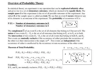
Overview of Probability TheoryIn statistical theory, an experiment is any operation that can be replicated infinitely often and gives rise to a set of elementary outcomes, which are deemed to be equally likely. The sample space S of the experiment is the set of all possible outcomes of the experiment. Any subset E of the sample space is called an event. We say that an event E occurs whenever any of its elements is an outcome of the experiment. The probability of occurrence of E is P {E} = Number of elementary outcomes in E Number of elementary outcomes in SThe complement E of an event E is the set of all elements that belong to S but not to E. The union of two events E1 E2 is the set of all outcomes that belong to E1 or to E2 or to both. The intersection of two events E1 E2 is the set of all events that belong to both E1 and E2.Two events are mutually exclusive if the occurrence of either precludes the occurrence of the other (i.e) their intersection is the empty set . Two events are independent if the occurrence of either is unaffected by the occurrence or non-occurrence of the other event.Theorem of Total Probability. P {E1 E2} = P{E1} + P{E2} - P{E1 E2}Proof. P{E1 E2} = (n1, 0 + n1, 2 + n0, 2) / n = (n1, 0 + n1, 2) / n + (n1, 2 + n0, 2) / n - n1, 2 / n = P{E1} + P{E2} - P{E1 E2}Corollary.If E1 and E2 are mutually exclusive, P{E1 E2} = P{E1} + P{E2} S E S n = n0, 0 + n1, 0 + n0, 2 + n1, 2 E1 E2 n1, 0 n1, 2 n0, 2 n0, 0
The probability P{E1 | E2} thatE1 occurs, given that E2 has occurred (or must occur) is called the conditional probability of E1. Note that in this case, the only possible outcomes of the experiment are confined to E2 and not to S.Theorem of Compound ProbabilityP{E1 E2} = P{E1 | E2} * P{E2}.Proof. P{E1 E2} = n1, 2 / n = {n1, 2 / (n1, 2 + n0, 2) } * { n1, 2 + n0, 2) / n} Corollary.If E1 and E2 are independent, P{E1 E2} = P{E1} * P{E2}. The ability to count the possible outcomes in an event is crucial to calculating probabilities. By a permutation of size r of n different items, we mean an arrangement of r of the items, where the order of the arrangement is important. If the order is not important, the arrangement is called a combination.Example. There are 5*4 permutations and 5*4 / (2*1) combinations of size 2 of A, B, C, D, EPermutations: AB, BA, AC, CA, AD, DA, AE, EA BC, CB, BD, DB, BE, EB CD, DC, CE, EC DE, EDCombinations: AB, AC, AD, AE, BC, BD, BE, CD, CE, DEStandard reference books on probability theory give a comprehensive treatment of how these ideas are used to calculate the probability of occurrence of the outcomes of games of chance. S E2 E1 n1, 0 n1, 2 n0, 2 n0, 0
Statistical DistributionsIf a statistical experiment only gives rise to real numbers, the outcome of the experiment is called a random variable. If a random variable X takes values X1, X2, … , Xn with probabilities p1, p2, … , pnthen the expected or average value of X is defined to be E[X] = pj Xj and its variance is VAR[X] = E[X2] - (E[X])2 = pj Xj2 - (E[X])2. Example. Let X be a random variable measuring Prob. Distancethe distance in Kilometres travelled by children pj Xj pj Xj pj Xj2to a school and suppose that the following data applies. Then the mean and variance are 0.15 2.0 0.30 0.60 E[X] = 5.30 Kilometres 0.40 4.0 1.60 6.40 VAR[X] = 33.80 - 5.302 0.20 6.0 1.20 7.20 = 5.71 Kilometres2 0.15 8.0 1.20 9.60 0.10 10.0 1.00 1.00 1.00 - 5.30 33.80 Similar concepts apply to continuous distributions. The distribution function is defined by F(t) = P{ X t} and its derivative is the frequency function f(t) = d F(t) / dt so that F(t) = f(x) dx.
Sums and Differences of Random VariablesDefine the covariance of two random variables to be COVAR [ X, Y] = E [(X - E[X]) (Y - E[Y]) ] = E[X Y] - E[X] E[Y].If X and Y are independent, COVAR [X, Y] = 0.Lemma E[ X + Y] = E[X] + E[Y] VAR [ X + Y] = VAR [X] + VAR [Y] + 2 COVAR [X, Y] E[ k. X] = k .E[X] VAR[ k. X] = k2 .VAR[X] for a constant k.Example. A company records the journey time X X=1 2 3 4 Totalsof a lorry from a depot to customers and Y =1 7 5 4 4 20 the unloading times Y, as shown. 2 2 6 8 3 19E[X] = {1(10)+2(13)+3(17)+4(10)}/50 = 2.54 3 1 2 5 3 11E[X2] = {12(10+22(13)+32(17)+42(10)}/50 = 7.5 Totals 10 13 17 10 50 VAR[X] = 7.5 - (2.54)2 = 1.0484E[Y] = {1(20)+2(19)+3(11)}/50 = 1.82 E[Y2] = {12(20)+22(19)+32(11)}/50 = 3.9VAR[Y] = 3.9 - (1.82)2 = 0.5876 E[X+Y] = { 2(7)+3(5)+4(4)+5(4)+3(2)+4(6)+5(8)+6(3)+4(1)+5(2)+6(5)+7(3)}/50 = 4.36 E[(X + Y)2] = {22(7)+32(5)+42(4)+52(4)+32(2)+42(6)+52(8)+62(3)+42(1)+52(2)+62(5)+72(3)}/50 = 21.04VAR[(X+Y)] = 21.04 - (4.36)2 = 2.0304 E[X.Y] = {1(7)+2(5)+3(4)+4(4)+2(2)+4(6)+6(8)+8(3)+3(1)+6(2)+9(5)+12(3)}/50 = 4.82COVAR (X, Y) = 4.82 - (2.54)(1.82) = 0.1972VAR[X] + VAR[Y] + 2 COVAR[ X, Y] = 1.0484 + 0.5876 + 2 ( 0.1972) = 2.0304