Modeling Fluid Phenomena
Modeling Fluid Phenomena. Vinay Bondhugula (25 th & 27 th April 2006). Two major techniques. Solve the PDE describing fluid dynamics. Simulate the fluid as a collection of particles. Rapid Stable Fluid Dynamics for Computer Graphics – Kass and Miller SIGGRAPH 1990. Previous Work.

Modeling Fluid Phenomena
E N D
Presentation Transcript
Modeling Fluid Phenomena Vinay Bondhugula (25th & 27th April 2006)
Two major techniques • Solve the PDE describing fluid dynamics. • Simulate the fluid as a collection of particles.
Rapid Stable Fluid Dynamics for Computer Graphics – Kass and Miller SIGGRAPH 1990
Previous Work • Older techniques were not realistic enough: • Tracking of individual waves • No net transport of water • Can’t handle changes in boundary conditions
Introduction • Approximates wave equation for shallow water. • Solves the wave equation using implicit integration. • The result is good enough for animation purposes.
Shallow Water Equations: Assumptions • Represent water by a height field. Motivation: • In an accurate simulation, computational cost grows as the cube of resolution. Limitation: • No splashing of water. • Waves cannot break.
Contd… 2) Ignore the vertical component of the velocity of water. Limitation: Inaccurate simulation for steep waves.
Contd… 3) Horizontal component of the velocity in a column is constant. Assumption fails in some cases: • Undercurrent • Greater friction at the bottom.
Notation • h(x) is the height of the water surface • b(x) is the height of the ground surface • d(x) = h(x) – b(x) is the depth of the water • u(x) is the horizontal velocity of a vertical water column. • di(n) is the depth at the ith point after the nth iteration.
The Equations • F = ma, gives the following: The second term is the horizontal force acting on a water column. • Volume conservation gives:
Contd… • Differentiating equation 1 w.r.t x and equation 2 w.r.t t we get: • From the simplified wave equation, the wave velocity is sqrt(gd). • Explains why tsunami waves are high • The wave slows down as it approaches the coast, which causes water to pile up.
Discretization • Finite-difference technique is applied:
Integration • Implicit techniques are used:
Another approximation • Still a non-linear equation! • ‘d’ is dependent on ‘h’ • Assume ‘d’ to be constant during integration • Wave velocities only change between iterations.
The linear equation: • Symmetric tridiagonal matrices can be solved very efficiently.
The linear equation • The linear equation can be considered an extrapolation of the previous motion of the fluid. • Damping can be introduced if the equation is written as:
A Subtle Issue • In an iteration, nothing prevents h from becoming less than b at a particular point, leading to negative volume at that point. • To compensate for this the iteration creates volume elsewhere (note that our equations conserve volume). • Solution: After each iteration, compute the new volume and compare it with the old volume.
The Equation in 3D • Split the equation into two terms - one independent of x and the other independent of y - and solve it in two sub-iterations. • We still obtain a linear system!
Rendering • Rendered with caustics – the terrain was assumed to be flat. • Real-time simulation!! • 30 fps on a 32x32 grid
Miscellaneous • Walls are simulated by having a steep incline.
Results Water flowing down a hill…
More Images Wave speed depends on the depth of the water…
Particle-Based Fluid Simulation for Interactive Applications • Matthias Muller et. al. SCA 2003
Motivation Limitations of grid based simulation: • No splashing or breaking of waves • Cannot handle multiple fluids • Cannot handle multiple phases
Introduction • Use Smoothed Particle Hydrodynamics (SPH) to simulate fluids with free surfaces. • Pressure and viscosity are derived from the Navier-Stokes equation. • Interactive simulation (about 5 fps).
SPH • Originally developed for astrophysical problems (1977). • Interpolation method for particles. • Properties that are defined at discrete particles can be evaluated anywhere in space. • Uses smoothing kernels to distribute quantities.
Contd… • mjis the mass, rj is the density, Aj is the quantity to be interpolated and W is the smoothing kernel
Modeling Fluids with Particles • Given a control volume, no mass is created in it. Hence, all mass that comes out has to be accounted by change in density. But, mass conservation is anyway guaranteed in a particle system.
Contd… • Momentum equation: Three components: • Pressure term • Force due to gravity • Viscosity term (m is the viscosity of the liquid)
Pressure Term • It’s not symmetric! Can easily be observed when only two particles interact. • Instead use this: • Note that the pressure at each particle is computed first. Use the ideal gas state equation: p = k*r, where k is a constant which depends on the temperature.
Viscosity Term • Method used is similar to the one used for the pressure term.
Miscellaneous • Other external forces are directly applied to the particles. • Collisions: In case of collision the normal component of the velocity is flipped.
Smoothing Kernel • Has an impact on the stability and speed of the simulation. • eg. Avoid square-roots for distance computation. • Sample smoothing kernel: all points inside a radius of ‘h’ are considered for “smoothing”.
Surface Tracking and Visualization • Define a quantity that is 1 at particle locations and 0 elsewhere (it’s called the color field). • Smooth it out: • Compute the gradient of this field:
Contd… • If |n(ri)| > l, then the point is a surface point. • l is a threshold parameter.
Results • Interactive Simulation (5fps) • Videos from Muller’s site: http://graphics.ethz.ch/~mattmuel/
References • Rapid, Stable Fluid Dynamics for Computer Graphics – Michael Kass and David Miller – SIGGRAPH 1990 • Particle-Based Fluid Simulation for Interactive Applications – Muller et. al., SCA 2003 • Particle-Based Fluid-Fluid Interaction - M. Muller, B. Solenthaler, R. Keiser, M. Gross – SCA 2005