Download
1 / 15
160 likes | 214 Vues
Ch3-Sec(3.5): Nonhomogeneous Equations; Method of Undetermined Coefficients. Recall the nonhomogeneous equation where p , q, g are continuous functions on an open interval I . The associated homogeneous equation is

E N D
Ch3-Sec(3.5): Nonhomogeneous Equations; Method of Undetermined Coefficients • Recall thenonhomogeneous equation where p, q,g are continuous functions on an open interval I. • The associated homogeneous equation is • In this section we will learn the method of undetermined coefficients to solve the nonhomogeneous equation, which relies on knowing solutions to the homogeneous equation.
Theorem 3.5.1 • If Y1 and Y2 are solutions of the nonhomogeneous equation then Y1 -Y2 is a solution of the homogeneous equation • If, in addition, {y1, y2} forms a fundamental solution set of the homogeneous equation, then there exist constants c1 and c2 such that
Theorem 3.5.2 (General Solution) • The general solution of the nonhomogeneous equation can be written in the form where y1 and y2 form a fundamental solution set for the homogeneous equation, c1 and c2 are arbitrary constants, and Y(t) is a specific solution to the nonhomogeneous equation.
Method of Undetermined Coefficients • Recall the nonhomogeneous equation with general solution • In this section we use the method of undetermined coefficients to find a particular solution Y to the nonhomogeneous equation, assuming we can find solutions y1, y2 for the homogeneous case. • The method of undetermined coefficients is usually limited to when p and q are constant, and g(t) is a polynomial, exponential, sine or cosine function.
Example 1: Exponential g(t) • Consider the nonhomogeneous equation • We seek Y satisfying this equation. Since exponentials replicate through differentiation, a good start for Y is: • Substituting these derivatives into the differential equation, • Thus a particular solution to the nonhomogeneous ODE is
Example 2: Sine g(t), First Attempt (1 of 2) • Consider the nonhomogeneous equation • We seek Y satisfying this equation. Since sines replicate through differentiation, a good start for Y is: • Substituting these derivatives into the differential equation, • Since sin(x) and cos(x) are not multiples of each other, we must have c1= c2 = 0, and hence 2 + 5A = 3A = 0, which is impossible.
Example 2: Sine g(t), Particular Solution (2 of 2) • Our next attempt at finding a Y is • Substituting these derivatives into ODE, we obtain • Thus a particular solution to the nonhomogeneous ODE is
Example 3: Product g(t) • Consider the nonhomogeneous equation • We seek Y satisfying this equation, as follows: • Substituting these into the ODE and solving for A and B:
Discussion: Sum g(t) • Consider again our general nonhomogeneous equation • Suppose that g(t) is sum of functions: • If Y1, Y2 are solutions of respectively, then Y1 + Y2 is a solution of the nonhomogeneous equation above.
Example 4: Sum g(t) • Consider the equation • Our equations to solve individually are • Our particular solution is then
Example 5: First Attempt (1 of 3) • Consider the nonhomogeneous equation • We seek Y satisfying this equation. We begin with • Substituting these derivatives into differential equation, • Since the left side of the above equation is always 0, no value of A can be found to make a solution to the nonhomogeneous equation. • To understand why this happens, we will look at the solution of the corresponding homogeneous differential equation
Example 5: Homogeneous Solution (2 of 3) • To solve the corresponding homogeneous equation: • We use the techniques from Section 3.1 and get • Thus our assumed particular solution solves the homogeneous equation instead of the nonhomogeneous equation. • So we need another form for Y(t) to arrive at the general solution of the form:
Example 5: Particular Solution (3 of 3) • Our next attempt at finding a Y(t) is: • Substituting these into the ODE, • So the general solution to the IVP is
Summary – Undetermined Coefficients (1 of 2) • For the differential equation where a, b, and c are constants, if g(t) belongs to the class of functions discussed in this section (involves nothing more than exponential functions, sines, cosines, polynomials, or sums or products of these), the method of undetermined coefficients may be used to find a particular solution to the nonhomogeneous equation. • The first step is to find the general solution for the corresponding homogeneous equation with g(t) = 0.
Summary – Undetermined Coefficients (2 of 2) The second step is to select an appropriate form for the particular solution, Y(t), to the nonhomogeneous equation and determine the derivatives of that function. After substituting Y(t), Y’(t), and Y”(t) into the nonhomo-geneous differential equation, if the form for Y(t) is correct, all the coefficients in Y(t) can be determined. Finally, the general solution to the nonhomogeneous differential equation can be written as