Asymptotic Notation in Algorithm Analysis
This informative guide covers the basics of asymptotic notation, focusing on Divide-and-Conquer Approach, Merge Sort Algorithm, Θ-notation, O-notation, Ω-notation, and more. Learn how to analyze algorithms effectively.

Asymptotic Notation in Algorithm Analysis
E N D
Presentation Transcript
Asymptotic Notation CS 583 Analysis of Algorithms CS583 Fall'06: Asymptotic Notation
Outline • Divide-and-Conquer Approach • Merge Sort Algorithm • Pseudocode • Asymptotic Notation • -notation • O-notation • -notation, etc. • Randomized Algorithms CS583 Fall'06: Asymptotic Notation
Divide-and-Conquer Approach • Break the problem into several subproblems that are similar to the original problem, but smaller in size; solve the subproblems recursively; then combine the solutions. • Divide the problem into a number of subproblems. • Conquer the subproblems by solving them recursively. • Combine he solutions into the solution of the original problem. CS583 Fall'06: Asymptotic Notation
Merge Sort Algorithm • Divide an n-element sequence to be sorted into two n/2-subsequences. • Sort the two subsequences recursively using merge sort. • Merge two subsequences to get the sorted answer. • The key procedure is to merge A[p..q] with A[q+1..r] assuming both sequences are sorted. • Two arrays are merged by moving the smaller of two numbers to the resulting array at each step. There are at most n steps performed, so merging takes (n) time. • A special sentinel number (max_int) is placed at the bottom to simplify the comparison. CS583 Fall'06: Asymptotic Notation
Merge Sort: Pseudocode MERGE (A, p, q, r) 1 n1 = q-p+1 2 n2 = r-q 3 // create left and right arrays 4 for i=1 to n1 5 L[i] = A[p+i-1] 6 for i=1 to n2 7 R[i] = A[q+i] 8 L[n1+1] = max_int 9 R[n2+1] = max_int 10 i=1 11 j=1 12 for k=p to r 13 if L[i] <= R[j] 14 A[k]=L[i] 15 i = i+1 16 else 17 A[k]=R[j] 18 j = j+1 CS583 Fall'06: Asymptotic Notation
Merge Sort: Pseudocode (cont.) The main merge sort procedure sorts elements in the subarray A[p..r]: MERGE-SORT-RUN (A, p, r) 1 if p<r 2 q = ceil((p+r)/2) 3 MERGE-SORT-RUN(A,p,q) 4 MERGE-SORT-RUN(A,q+1,r) 5 MERGE(A,p,q,r) The merge sort algorithm simply runs the main procedure on an array A[1..n]: MERGE-SORT (A, n) 1 MERGE-SORT-RUN(A,1,n) CS583 Fall'06: Asymptotic Notation
Merge Sort: Analysis • Assume the original problem's size n=2x. • The divide step just computes the middle of an array • This takes constant time: c. • We solve two subproblems, each of size n/2. • Combining is a merge procedure that takes (n) time. c, if n = 1 T(n) = 2T(n/2)+ cn, otherwise There are lg(n) recursive steps, each takes cn time: T(n) = cnlg(n) CS583 Fall'06: Asymptotic Notation
Asymptotic Notation • The notations are defined in terms of functions whose domains are the set of natural numbers N={0,1,2,...}. • Such notations are convenient for describing the worst-case running time function T(n). • It can also be extended to the domain of real numbers. CS583 Fall'06: Asymptotic Notation
-notation For a given function g(n) we denote by (g(n)) the set of functions: (g(n)) = {f(n): c1, c2, n0 > 0 ( n>= n0 0 <= c1 g(n) <= f(n) <= c2 g(n)))} f(n) = (g(n)) f(n) (g(n)) g(n) is an asymptotically tight bound for f(n) CS583 Fall'06: Asymptotic Notation
(n/100+100) = (n) Find c1, c2, n0 such that c1n <= n/100+100<=c2n for all n>=n0 c1 <= 1/100 + 100/n <= c2 For n=n0=1 we have: c1 <= 100 + 1/100 c2 >= 100 + 1/100 Choose c1 = 1/100; c2= 100.001, then the above equation will hold for any n>=1. -notation: Examples CS583 Fall'06: Asymptotic Notation
f(n)=1000 (n) By contradiction, suppose there is c1 so that c1n <= 1000 for all n>=n0 n <= 1000/c1, which cannot hold for arbitrarily large n since c1 is constant. -notation: Examples (cont.) CS583 Fall'06: Asymptotic Notation
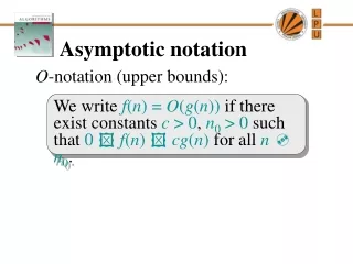
O-notation We use O-notation when we have only an asymptotic upper bound: O(g(n)) = {f(n) : c,n0 > 0 ( n>= n0 (0 <= f(n) <= cg(n)))} Note that, (g(n)) O(g(n)). For example, n = O(n2). Since O-notation describes an upper bound, when we use it to bound the worst-case running time of an algorithm, we have a bound on every input. For example, the O(n2) bound on the insertion sort also applies to its running time on every input However, (n2) on the insertion sort would only apply to the worst-case input. CS583 Fall'06: Asymptotic Notation
-notation -notation provides an asymptotic lower bound n a function: (g(n)) = {f(n) : c,n0 > 0 ( n>= n0 (0 <= cg(n) <= f(n)))} Since -notation describes a lower bound, it is useful when applied to the best-case running time of algorithms. For example, the best-case running time of the insertion sort is (n), which implies that the running time of insertion sort (n). CS583 Fall'06: Asymptotic Notation
o-notation This notation is used to denote an upper bound that is not asymptotically tight: o(g(n))={f(n) : c > 0 ( n0>0 (0 <= f(n) <= cg(n) for all n>n0))} For example, 2n = o(n2). Intuitively: lim f(n)/g(n) = 0 CS583 Fall'06: Asymptotic Notation
-notation We use -notation to denote a lower bound that is not asymptotically tight: (g(n))={f(n) : c > 0 ( n0>0 (0 <= cg(n) <= f(n) for all n>n0))} For example, n2/2 = (n). The relationship implies: lim f(n)/g(n) = CS583 Fall'06: Asymptotic Notation
The Hiring Problem • The goal is to hire a new assistant through an employment agency. • The agency sends one candidate each day. • The commitment is to have the best person to do the job. • When the interviewed person is better than the current assistant, he/she is hired in place of the current one. • There is a small cost to pay for the interview. • There is usually a larger cost associated with the fire/hire process. CS583 Fall'06: Asymptotic Notation
The Hiring Problem: Algorithm • Hire-Assistant (n) • 1 best = 0 // candidate 0 is least qualified • 2 for i = 1 to n • <interview candidate i> • 4 ifi is better than best • 5 best = i • 6 <hire candidate i> • Assume interviewing has cost ci, whereas more expensive hiring has cost ch. Let m be the number of people hired. Then the cost of the above algorithm is: • O(nci + mch) • The quantity m varies with each run and determines the overall cost of the algorithm. It is estimated using probabilistic analysis. CS583 Fall'06: Asymptotic Notation
Indicator Random Variables Assume sample space S and an event A. The indicator random variable I{A} is defined as 1, if A occurs I{A} = 0, otherwise Given a sample space S and an event A, denote XA a random variable associated with an event being A, i.e. XA = I{A}. The the expected value of XA is: E[XA] = Pr{A} Proof. E[XA] = E[I{A}] = 1Pr{A} + 0Pr{A} = Pr{A} CS583 Fall'06: Asymptotic Notation
The Hiring Problem: Analysis Let Xi be the indicator random variable associated with the event that the candidate i is hired: Xi = I{candidate i is hired} Let X be the random variable whose value equals the number of time we hire a new candidate: X = X1 + ... + Xn Note that E[Xi] = Pr{Xi} = Pr{candidate i is hired}. We now need to compute Pr{candidate i is hired}. CS583 Fall'06: Asymptotic Notation
The Hiring Problem: Analysis (cont.) Candidate i is hired (line 5) when it is better than any of the previous (i-1) candidates. Since all candidates arrive in random order, each of them have the same probability of being the best so far. Therefore: E[Xi] = Pr{Xi} = 1/i We can now compute E[X]: E[X] = E[X1 + ... + Xn] = 1 + ½ + ... + 1/n = ln(n) + O(1) Hence, when candidates are presented in random order, the algorithm Hire-Assistant has a total hiring cost: O(ch ln(n)) CS583 Fall'06: Asymptotic Notation
Randomized Algorithms In a randomized algorithm the distribution of inputs is imposed. In particular, in the randomized version of the Hire-Assistant algorithm we randomly permute the candidates: Randomized-Hire-Assistant (n) 1 <randomly permute the list of candidates> 2 best = 0 // candidate 0 is least qualified 3 for i = 1 to n 4 <interview candidate i> 5 ifi is better than best 6 best = i 7 <hire candidate i> According to the earlier computations, the expected cost of the above algorithm is O(nci+chln(n)). CS583 Fall'06: Asymptotic Notation