Asymptotic Analysis
Asymptotic Analysis. Outline. 2.3. In this topic, we will look at: Justification for analysis Quadratic and polynomial growth Counting machine instructions Landau symbols Big- Q as an Equivalence Relation Little- o as a Linear Ordering. Background. 2.3.


Asymptotic Analysis
E N D
Presentation Transcript
Outline 2.3 In this topic, we will look at: • Justification for analysis • Quadratic and polynomial growth • Counting machine instructions • Landau symbols • Big-Q as an Equivalence Relation • Little-o as a Linear Ordering
Background 2.3 Suppose we have two algorithms, how can we tell which is better? We could implement both algorithms, run them both • Expensive and error prone Preferably, we should analyze them mathematically • Algorithm analysis
Asymptotic Analysis 2.3.1 In general, we will always analyze algorithms with respect to one or more variables We will begin with one variable: • The number of items n currently stored in an array or other data structure • The number of items expected to be stored in an array or other data structure • The dimensions of an n ×n matrix Examples with multiple variables: • Dealing with n objects stored in m memory locations • Multiplying a k ×m and an m ×n matrix • Dealing with sparse matrices of size n ×n with m non-zero entries
Maximum Value 2.3.1 For example, the time taken to find the largest object in an array of n random integers will take n operations int find_max( int *array, int n ) { int max = array[0]; for ( int i = 1; i < n; ++i ) { if ( array[i] > max ) { max = array[i]; } } return max; }
Maximum Value 2.3.1 One comment: • In this class, we will look at both simple C++ arrays and the standard template library (STL) structures • Instead of using the built-in array, we could use the STL vector class • The vector class is closer to the C#/Java array
Maximum Value 2.3.1 #include <vector> intfind_max( std::vector<int> array ) { if ( array.size() == 0 ) { throw underflow(); } int max = array[0]; for ( inti = 1; i < array.size(); ++i ) { if ( array[i] > max ) { max = array[i]; } } return max; }
Linear and binary search There are other algorithms which are significantly faster as the problem size increases This plot shows maximumand average number ofcomparisons to find an entryin a sorted array of size n Linear search Binary search 2.3.2 n
Asymptotic Analysis 2.3.3 Given an algorithm: • We need to be able to describe these values mathematically • We need a systematic means of using the description of the algorithm together with the properties of an associated data structure • We need to do this in a machine-independent way For this, we need Landau symbols and the associated asymptotic analysis
Quadratic Growth 2.3.3 Consider the two functions f(n) = n2 and g(n) = n2 – 3n + 2 Around n = 0, they look very different
Quadratic Growth 2.3.3 Yet on the range n = [0, 1000], they are (relatively) indistinguishable:
Quadratic Growth 2.3.3 The absolute difference is large, for example, f(1000) = 1 000 000 g(1000) = 997 002 but the relative difference is very small and this difference goes to zero as n →∞
Polynomial Growth 2.3.3 To demonstrate with another example, f(n) = n6 and g(n) = n6 – 23n5+193n4 –729n3+1206n2 – 648n Around n = 0, they are very different
Polynomial Growth 2.3.3 Still, around n = 1000, the relative difference is less than 3%
Polynomial Growth 2.3.3 The justification for both pairs of polynomials being similar is that, in both cases, they each had the same leading term: n2 in the first case, n6 in the second Suppose however, that the coefficients of the leading terms were different • In this case, both functions would exhibit the same rate of growth, however, one would always be proportionally larger
Examples 2.3.4 We will now look at two examples: • A comparison of selection sort and bubble sort • A comparison of insertion sort and quicksort
Counting Instructions 2.3.4.1 Suppose we had two algorithms which sorted a list of size n and the run time (in ms) is given by bworst(n) = 4.7n2 – 0.5n + 5Bubble sort bbest(n) = 3.8n2 + 0.5n + 5 s(n) = 4n2 + 14n + 12 Selection sort The smaller the value, the fewer instructions are run • For n≤ 21, bworst(n) < s(n) • For n≥ 22, bworst(n) > s(n)
Counting Instructions 2.3.4.1 With small values of n, the algorithm described by s(n)requires more instructions than even the worst-case for bubble sort
Counting Instructions 2.3.4.1 Near n = 1000, bworst(n) ≈ 1.175 s(n) and bbest(n) ≈ 0.95 s(n)
Counting Instructions 2.3.4.1 Is this a serious difference between these two algorithms? Because we can count the number instructions, we can also estimate how much time is required to run one of these algorithms on a computer
Counting Instructions 2.3.4.1 Suppose we have a 1 GHz computer • The time (s) required to sort a list of up to n = 10 000 objects is under half a second
Counting Instructions 2.3.4.1 To sort a list with one million elements, it will take about 1h Bubble sort could, under some conditions, be 200 s faster
Counting Instructions 2.3.4.1 How about running selection sort on a faster computer? • For large values of n, selection sort on a faster computer will always be faster than bubble sort
Counting Instructions 2.3.4.1 Justification? • If f(n) = aknk + ··· and g(n) = bknk + ···, for large enough n, it will always be true that f(n) < Mg(n) where we choose M = ak/bk + 1 In this case, we only need a computer which is M times faster (or slower) Question: • Is a linear search comparable to a binary search? • Can we just run a linear search on a slower computer?
Counting Instructions 2.3.4.2 As another example: • Compare the number of instructions required for insertion sort and for quicksort • Both functions are concave up, although one more than the other
Counting Instructions 2.3.4.2 Insertion sort, however, is growing at a rate of n2 while quicksort grows at a rate of nlg(n) • Never-the-less, the graphic suggests it is more useful to use insertion sort when sorting small lists—quicksort has a large overhead
Counting Instructions 2.3.4.2 If the size of the list is too large (greater than 20), the additional overhead of quicksort quickly becomes insignificant • The quicksort algorithm becomes significantly more efficient • Question: can we just buy a faster computer?
Landau Symbols 2.3.5 Recall Landau symbols from 1st year: A function f(n) = O(g(n)) if there exists N and c such that f(n) < c g(n) whenever n > N • The function f(n) has a rate of growth no greater than that of g(n)
Landau Symbols 2.3.5 Before we begin, however, we will make some assumptions: • Our functions will describe the time or memory required to solve a problem of size n • We conclude we are restricting ourselves to certain functions: • They are defined for n ≥ 0 • They are strictly positive for all n • In fact, f(n) > c for some value c > 0 • That is, any problem requires at least one instruction and byte • They are increasing (monotonic increasing)
Landau Symbols 2.3.5 Another Landau symbol is Q A function f(n) = Q(g(n)) if there exist positive N, c1, and c2 such that c1g(n) < f(n) < c2g(n) whenever n > N • The function f(n) has a rate of growth equal to that of g(n)
Landau Symbols 2.3.5 These definitions are often unnecessarily tedious Note, however, that if f(n) and g(n) are polynomials of the same degree with positive leading coefficients: where
Landau Symbols 2.3.5 Suppose that f(n) and g(n) satisfy From the definition, this means given c > e > 0 there exists an N > 0 such that whenever n > N That is,
Landau Symbols 2.3.5 However, the statementsays that f(n) = Q(g(n)) Note that this only goes one way: If where , it follows that f(n) = Q(g(n))
Landau Symbols 2.3.6 We have a similar definition for O: If where , it follows that f(n) = O(g(n)) There are other possibilities we would like to describe: If , we will say f(n) = o(g(n)) • The function f(n) has a rate of growth less than that of g(n) We would also like to describe the opposite cases: • The function f(n) has a rate of growth greater than that of g(n) • The function f(n) has a rate of growth greater than or equal to that of g(n)
Asymptotic Analysis 2.3.7 We will at times use five possible descriptions
Landau Symbols 2.3.7 For the functions we are interested in, it can be said that f(n) = O(g(n)) is equivalent to f(n) = Q(g(n)) or f(n) = o(g(n)) and f(n) = W(g(n)) is equivalent to f(n) = Q(g(n)) or f(n) = w(g(n))
Landau Symbols 2.3.7 Graphically, we can summarize these as follows: We say if
Landau Symbols 2.3.8 Some other observations we can make are: f(n) = Q(g(n)) ⇔ g(n) = Q(f(n)) f(n) = O(g(n)) ⇔ g(n) = W(f(n)) f(n) = o(g(n)) ⇔ g(n) = w(f(n))
Big-Q as an Equivalence Relation 2.3.8 If we look at the first relationship, we notice thatf(n) = Q(g(n)) seems to describe an equivalence relation: 1. f(n) = Q(g(n)) if and only if g(n) = Q(f(n)) 2. f(n) = Q(f(n)) 3. If f(n) = Q(g(n)) and g(n) = Q(h(n)), it follows that f(n) = Q(h(n)) Consequently, we can group all functions into equivalence classes, where all functions within one class are big-theta Q of each other
Big-Q as an Equivalence Relation 2.3.8 For example, all of n2 100000 n2 – 4 n + 19 n2 + 1000000 323 n2 – 4 n ln(n) + 43 n + 10 42n2 + 32 n2 + 61 n ln2(n) + 7n + 14 ln3(n) + ln(n) are big-Q of each other E.g., 42n2 + 32 = Q( 323 n2 – 4 n ln(n) + 43 n + 10 )
Big-Q as an Equivalence Relation 2.3.8 Recall that with the equivalence class of all 19-year olds, we only had to pick one such student? Similarly, we will select just one element to represent the entire class of these functions: n2 • We could chose any function, but this is the simplest
Big-Q as an Equivalence Relation 2.3.8 The most common classes are given names: Q(1) constant Q(ln(n)) logarithmic Q(n) linear Q(n ln(n)) “n log n” Q(n2) quadratic Q(n3) cubic 2n, en, 4n, ...exponential
Logarithms and Exponentials 2.3.8 Recall that all logarithms are scalar multiples of each other • Therefore logb(n)= Q(ln(n)) for any base b Alternatively, there is no single equivalence class for exponential functions: • If 1 < a < b, • Therefore an = o(bn) However, we will see that it is almost universally undesirable to have an exponentially growing function!
Logarithms and Exponentials 2.3.8 Plotting 2n,en, and 4n on the range [1, 10] already shows how significantly different the functions grow Note: 210 = 1024 e10 ≈ 22 026 410 = 1 048 576
Little-o as a Weak Ordering 2.3.9 We can show that, for example ln( n ) = o( np ) for any p > 0 Proof: Using l’Hôpital’s rule, we have Conversely, 1 = o(ln( n ))
Little-o as a Weak Ordering 2.3.9 Other observations: • If p and q are real positive numbers where p < q, it follows that np = o(nq) • For example, matrix-matrix multiplication is Q(n3) but a refined algorithm is Q(nlg(7)) where lg(7) ≈ 2.81 • Also, np = o(ln(n)np), but ln(n)np = o(nq) • np has a slower rate of growth than ln(n)np, but • ln(n)np has a slower rate of growth than nq for p < q
Little-o as a Weak Ordering 2.3.9 If we restrict ourselves to functions f(n) which are Q(np) and Q(ln(n)np), we note: • It is never true that f(n) = o(f(n)) • If f(n) ≠ Q(g(n)), it follows that either f(n) = o(g(n)) or g(n) = o(f(n)) • If f(n) = o(g(n)) and g(n) = o(h(n)), it follows that f(n) = o(h(n)) This defines a weak ordering!
Little-o as a Weak Ordering 2.3.9 Graphically, we can shown this relationship by marking these against the real line
Algorithms Analysis 2.3.10 We will use Landau symbols to describe the complexity of algorithms • E.g., adding a list of n doubles will be said to be a Q(n) algorithm An algorithm is said to have polynomial time complexity if its run-time may be described by O(nd) for some fixed d ≥ 0 • We will consider such algorithms to be efficient Problems that have no known polynomial-time algorithms are said to be intractable • Traveling salesman problem: find the shortest path that visits ncities • Best run time: Q(n2 2n)
Algorithm Analysis 2.3.10 In general, you don’t want to implement exponential-time or exponential-memory algorithms • Warning: don’t call a quadratic curve “exponential”, either...please