Asymptotic Behavior
Asymptotic Behavior. Algorithm : Design & Analysis [2]. In the last class …. Goal of the Course Mathematical Background Probability Summations and Series Monotonic and Convex Functions Average and Worst-Case Analysis Lower Bounds and the Complexity of Problems. Asymptotic Behavior.


Asymptotic Behavior
E N D
Presentation Transcript
Asymptotic Behavior Algorithm : Design & Analysis [2]
In the last class… • Goal of the Course • Mathematical Background • Probability • Summations and Series • Monotonic and Convex Functions • Average and Worst-Case Analysis • Lower Bounds and the Complexity of Problems
Asymptotic Behavior • Asymptotic growth rate • The Sets , and • Complexity Class • An Example: Searching an Ordered Array • Improved Sequential Search • Binary Search • Binary Search Is Optimal
Fundamentals of Cost • Input • Input size: • Number of items (sorting) • Total number of bits (integer multiplying) • Number of vertices+number of edges (graph) • Structure of input • Running time • Number of primitive operations executed • Actual cost of each operation
How to Compare Two Algorithm? • Simplifying the analysis • assumption that the total number of steps is roughly proportional to the number of basic operations counted (a constant coefficient) • only the leading term in the formula is considered • constant coefficient is ignored • Asymptotic growth rate • large n vs. smaller n
Relative Growth Rate Ω(g):functions that grow at least as fast as g Θ(g):functions that grow at the same rate as g g Ο(g):functions that grow no faster as g
The Set “Big Oh” • Definition • Giving g:N→R+, then Ο(g) is the set of f:N→R+, such that for some cR+ and some n0N, f(n)cg(n) for all nn0. • A function fΟ(g) if limn→[f(n)/g(n)]=c< • Note: c may be zero. In that case, f(g), “little Oh” • Example: let f(n)=n2, g(n)=nlgn, then: • fΟ(g), since limn→[f(n)/g(n)]= limn→[n2/nlgn]= limn→[n/lgn]= limn→[1/(1/nln2)]= • gΟ(f), since limn→[g(n)/f(n)]=0
The Sets and • Definition • Giving g:N→R+, then (g) is the set of f:N→R+, such that for some cR+ and some n0N, f(n)cg(n) for all nn0. • A function f(g) if limn→[f(n)/g(n)]>0 • Note: the limit may be infinity • Definition • Giving g:N→R+, then (g) = Ο(g) (g) • A function fΟ(g) if limn→[f(n)/g(n)]=c,0<c<
Sorting a Array of 1 Million Numbers Using merge sort, taking time 50nlogn: 100 seconds! Computer B 10 Mips Computer A 1000 Mips Using insertion sort, taking time 2n2: 2000 seconds!
Properties of O, and • Transitive property: • If fO(g) and gO(h), then fO(h) • Symmetric properties • fO(g) if and only if g(f) • f(g) if and only if g(f) • Order of sum function • O(f+g)=O(max(f,g))
Complexity Class • Let S be a set of f:NR* under consideration, define the relation ~ on S as following: f~g iff. f(g) then, ~ is an equivalence. • Each set (g) is an equivalence class, called complexity class. • We usually use the simplest element as possible as the representative, so, (n), (n2), etc.
Comparison of Often Used Orders • The log function grows more slowly than any positive power of n lgn o(n) for any >0 • The power of n grows more slowly than any exponential function with base greater than 1 nk o(cn) for any c>1 (The commonly seen base is 2)
Order of Common Sums rk is the largest term in the sum f(n) Area=nf(n) f(rn) rn (0<r<1) n Area=(1-r)nf(rn)
. . . Roulette Wheel If there are W winners with bonus a, and L losers with penalty b, then the average winning will be: There are N slots , some winning and some losing 1 2 N 3 . . . i Winner: n
A Special Case with N=1000 Let winning bonus be 5, and losing penalty be 1
Solution Generalized Let the largest slot number be N, and , then:
Reasonable Approximation Now, we have: W=N/K+K2/2+5K/2-3, where K=
If Only N Large Enough… NW %error 1,000 10,000 100,000 1,000,000 10,000,000 100,000,000 1,000,000,000 150.0 696.2 3231.7 15000.0 69623.8 323165.2 1500000.0 172 746 3343 15247 70158 324322 1502497 12.791 6.670 3.331 1.620 0.761 0.357 0.166
Searching an Ordered Array • Problem: • Input: • an array E containing n entries of numeric type sorted in non-decreasing order • a value K • Output: • index for which K=E[index], if K is in E, or, -1, if K is not in E • Algorithm: • Int seqSearch(int[] E, int n, int K) • 1. Int ans, index; • 2. Ans=-1; // Assume failure • 3. For (index=0; index<n; index++) • 4. If (K==E[index]) ans=index;//success! • 5. break; • 6. return ans
gap(i-1) gap(i-1) gap(0) E[i] E[I+1] E[1] E[i-1] E[n] E[2] Searching a Sequence (cont.) • For a given K, there are two possibilities • K in E (say, with probability q), then K may be any one of E[i] (say, with equal probability, that is 1/n) • K not in E (with probability 1-q), then K may be located in any one of gap(i) (say, with equal probability, that is 1/(n+1))
Improved Sequential Search • Since E is sorted, when an entry larger than K is met, no more comparison is needed • Worst-case complexity: n, unchanged • Average complexity Note: A(n)(n) Roughly n/2
Divide and Conquer • If we compare K to every jth entry, we can locate the small section of E that may contain K. • To locate a section, roughly n/j steps at most • To search in a section, j steps at most • So, the worst-case complexity: (n/j)+j, with j selected properly, (n/j)+j(n) • However, we can use the same strategy in the small sections recursively Choose j = n
Binary Search int binarySearch(int[] E, int first, int last, int K) if (last<first) index=-1; else int mid=(first+last)/2 if (K==E[mid]) index=mid; else if (K<E[mid]) index=binarySearch(E, first, mid-1, K) else if (K<E[mid]) index=binarySearch(E, mid+1, last, K) return index;
Worst-case Complexity of Binary Search • Observation: with each call of the recursive procedure, only at most half entries left for further consideration. • At most lg n calls can be made if we want to keep the range of the section left not less than 1. • So, the worst-case complexity of binary search is lg n+1=lg(n+1)
Average Complexity of Binary Search • Observation: • for most cases, the number of comparison is or is very close to that of worst-case • particularly, if n=2k-1, all failure position need exactly k comparisons • Assumption: • all success position are equally likely (1/n) • n=2k-1
Average Complexity of Binary Search • Average complexity • Note: We count the sum of st, which is the number of inputs for which the algorithm does t comparisons, and if n=2k-1, st=2t-1
4 7 1 8 5 0 2 9 3 6 Decision Tree • An algorithms A that can do no other operations on the array entries except comparison can be modeled by a decision trees. • A decision tree for A and a given input of size n is a binary tree whose nodes are labeled with numbers between 0 and n-1 • Root: labeled with the index first compared • If the label on a particular node is i, then the left child is labeled the index next compared if K<E[i], the right child the index next compared if K>E[i], and no branch for the case of K=E[i].
Binary Search Is Optimal • If the number of comparison in the worst case is p, then the longest path from root to a leaf is p-1, so there are at most 2p-1 node in the tree. • There are at least n node in the tree. (We can prove that For all i{0,1,…,n-1}, exist a node with the label i.) • Conclusion: n 2p-1, that is plg(n+1)
Binary Search Is Optimal • For all i{0,1,…,n-1}, exist a node with the label i. • Proof: • if otherwise, suppose that i doesn’t appear in the tree, make up two inputs E1 and E2, with E1[i]=K, E2[i]=K’, K’>K, for any ji, (0jn-1), E1[j]=E2[j]. (Remember that both array are sorted). Since i doesn’t appear in the tree, for both K and K’, the algorithm behave alike exactly, and give the same outputs, of which at least one is wrong, so A is not a right algorithm.
Home Assignment • pp.63 – • 1.23 • 1.27 • 1.31 • 1.34 • 1.45