Asymptotic Growth Rates
200 likes | 515 Vues
Asymptotic Growth Rates. Themes Analyzing the cost of programs Ignoring constants and Big-Oh Recurrence Relations & Sums Divide and Conquer Examples Sort Computing powers Euclidean algorithm (computing gcds) Integer Multiplication. Asymptotic Growth Rates.

Asymptotic Growth Rates
E N D
Presentation Transcript
Asymptotic Growth Rates • Themes • Analyzing the cost of programs • Ignoring constants and Big-Oh • Recurrence Relations & Sums • Divide and Conquer • Examples • Sort • Computing powers • Euclidean algorithm (computing gcds) • Integer Multiplication
Asymptotic Growth Rates • f(n) = O(g(n)) [grows at the same rate or slower] • There exists positive constants c and n0 • such that f(n) c g(n) for all n n0 • Ignore constants and low order terms
Asymptotic Growth Rates (E.G.) • E.G. 1: 5n2 = O(n3) c = 1, n0= 5: 5n2 nn2 = n3 • E.G. 2: 100n2 = O(n2) c = 100, n0= 1 • E.G. 3: n3 = O(2n) c = 1, n0= 12 n3 (2n/3)3, n 2n/3 for n 12 [use induction]
Asymptotic Growth Rates • f(n) = o(g(n)) [grows slower] • f(n) = O(g(n)) and g(n) O(f(n)) • limn f(n)/g(n) = 0 • f(n) = (g(n)) [grows at the same rate] • f(n) = O(g(n)) and g(n) = O(f(n))
Asymptotic Growth Rates • [j < k] limn nj/nk = limn 1/n(k-j) = 0 • nj = o(nk) • [c < d] limn cn/dn = limn (c/d)n = 0 • cn = o(dn) • limn ln(n)/n = / • limn ln(n)/n = limn (1/n)/1 = 0 [L’Hopital’s Rule] • ln(n) = o(n) • [ > 0] ln(n) = o(n) [similar calculation]
Asymptotic Growth Rates • [c > 1, k an integer] • limn nk/cn = / • limn knk-1/ cnln(c) • limn k(k-1)nk-2/ cnln(c)2 • … • limn k(k-1)…(k-1)/cnln(c)k = 0 • nk = o(cn)
Asymptotic Growth Rates (E.G.) • limn f(n)/g(n) = 0 f(n) = O(g(n)) • >0, n0 s.t. n n0, f(n)/g(n) <
Asymptotic Growth Rates • (log(n)) – logarithmic [log(2n)/log(n) = 1 + log(2)/log(n)] • (n) – linear [double input double output] • (n2) – quadratic [double input quadruple output] • (n3) – cubit [double input output increases by factor of 8] • (nk) – polynomial of degree k • (cn) – exponential [double input square output]
Asymptotic Manipulation • (cf(n)) = (f(n)) • (f(n) + g(n)) = (f(n)) if g(n) = o(f(n))
Computing Time Functions • Computing time function is the time to execute a program as a function of its inputs • Typically the inputs are parameterized by their size [e.g. number of elements in an array, length of list, size of string,…] • Worst case = max runtime over all possible inputs of a given size • Best case = min runtime over all possible inputs of a given size • Average = avg. runtime over specified distribution of inputs
Analysis of Running Time • We can only know the cost up to constants through analysis of code [number of instructions depends on compiler, flags, architecture, etc.] • Assume basic statements are O(1) • Sum over loops • Cost of function call depends on arguments • Recursive functions lead to recurrence relations
Loops and Sums • for (i=0;i<n;i++) • for (j=i;j<n;j++) • S; // assume cost of S is O(1)
Merge Sort and Insertion Sort • Insertion Sort • TI(n) = TI(n-1) + O(n) =(n2) [worst case] • TI(n) = TI(n-1) + O(1) =(1) [best case] • Merge Sort • TM(n) = 2TM(n/2) + O(n) =(nlogn) [worst case] • TM(n) = 2TM(n/2) + O(n) =(nlogn) [best case]
Karatsuba’s Algorithm • Using the classical pen and paper algorithm two n digit integers can be multiplied in O(n2) operations. Karatsuba came up with a faster algorithm. • Let A and B be two integers with • A = A110k + A0, A0 < 10k • B = B110k + B0, B0 < 10k • C = A*B = (A110k + A0)(B110k + B0) = A1B1102k + (A1B0 + A0 B1)10k + A0B0 Instead this can be computed with 3 multiplications • T0 = A0B0 • T1 = (A1 + A0)(B1 + B0) • T2 = A1B1 • C = T2102k + (T1 - T0 - T2)10k + T0
Complexity of Karatsuba’s Algorithm • Let T(n) be the time to compute the product of two n-digit numbers using Karatsuba’s algorithm. Assume n = 2k. T(n) = (nlg(3)), lg(3) 1.58 • T(n) 3T(n/2) + cn 3(3T(n/4) + c(n/2)) + cn = 32T(n/22) + cn(3/2 + 1) 32(3T(n/23) + c(n/4)) + cn(3/2 + 1) = 33T(n/23) + cn(32/22 + 3/2 + 1) … 3iT(n/2i) + cn(3i-1/2i-1 + … + 3/2 + 1) ... cn[((3/2)k - 1)/(3/2 -1)] --- Assuming T(1) c 2c(3k - 2k) 2c3lg(n) = 2cnlg(3)
Divide & Conquer Recurrence Assume T(n) = aT(n/b) + (n) • T(n) = (n) [a < b] • T(n) = (nlog(n)) [a = b] • T(n) = (nlogb(a)) [a > b]