Chapter 2: Polynomial, Power, and Rational Functions

1. Section 2-3: Polynomial Functions of Higher Degree with Modeling Chapter 2:Polynomial, Power, and Rational Functions

2. Objectives • You will learn about: • Graphs of polynomial functions • End behavior of polynomial functions • Zeros of polynomial functions • Intermediate value theorem • Modeling • Why? • These topics are important in modeling and can be used to provide approximations to more complicated functions, as you will see if you study calculus.

3. Vocabulary • Cubic function • Quartic function • Term • Standard form • Coefficients • Leading term • Zoom out • Multiplicity m • Repeated zero • Polynomial interpolation

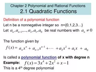
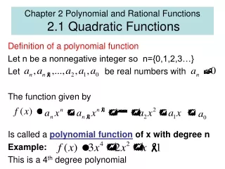
4. The Vocabulary of Polynomials • Each monomial in the sum anxn , an-1xn-1 ,…. a0 is a term of the polynomial. • A polynomial function written in this way, with terms in descending degree, is written in standard form. • The constants an ,an-1 , and a0 are the coefficients of the polynomial. • The term anxn is the leading term and a0 is the constant term.

5. Example 1Graphing Transformations of Monomial Functions • Describe how to transform the graph of an appropriate monomial function f(x)=anxninto the graph of the given function. • Sketch the graph • Compute the y-intercept

6. Example 2Graphing Combinations of Monomial Functions • Graph the polynomial function, locate its extrema and zeros. • Explain how it is related to the monomials from which it is built.

7. Graphs of Polynomial Functions • In general, graphs of polynomial functions: • Defined and continuous for all real numbers • Smooth, unbroken lines or curves; no sharp corners or cusps. • End behavior of polynomial functions– the end behavior of a polynomial is closely related to the end behavior of its leading term.

8. Exploration 1

9. Example 3Comparing the Graphs of Polynomials and its Leading Term • Superimpose the graphs of the polynomial and its leading term. • Then zoom out.

10. For all Polynomials • In sufficiently large viewing windows, the graph of a polynomial and the graph of its leading term appear to be identical. • The leading term dominates the behavior of the polynomial.

11. Leading Term Test for Polynomial End Behavior • For any polynomial function f(x) = anxn+… a1x1 + a0 the limits are determined by: • The degree n • The leading coefficient an

12. Example 4Applying Polynomial Theory • Graph the polynomial in a window showing its extrema, zeros, and end behavior. Describe the end behavior using limits.

13. Finding the Zeros of a Polynomial Function • Find the zeros of:

14. Multiplicity of a Zero of a Polynomial Function • If f is a polynomial function and (x – c)m is a factor but (x – c)m+1 is not, then c is a zero of multiplicity m of f. • A zero of multiplicity m ≥ 2 is a repeated zero.

15. Zeros of Odd and Even Multiplicity • If a polynomial function f has a real zero c of odd multiplicity, then the graph of f crosses the x-axis at (c,0) and the value of f changes sign at x = c. • If a polynomial function f has a real zero c of even multiplicity, then the graph of f does not cross the x-axis at (c,0) and the value of f does not change sign at x = c.

16. Example 6Sketching the Graph of a Factored Polynomial • State the degree and list the zeros of the function f(x) = (x+2)3 (x – 1)2

17. Theorem:Intermediate Value Theorem • If a and b are real numbers with a < b and f is continuous on the interval [a,b] then f takes on every value between f(a) and f(b). • In other words, if y0 is between f(a) and f(b), then y0 = f(c) for some number c in [a,b]. • In particular, if f(a) and f(b) have opposite signs, then f(c) for some c in [a,b].

18. Example 7Using the Intermediate Value Theorem • Explain why a polynomial function of odd degree has at least one real zero.

19. Example 8Zooming to Uncover Hidden Behavior • Find all the real zeros of:

20. Example 9Designing a Box • Dixie Packing Company has contracted to make boxes with a volume of approximately 484 in3. Squares are to be cut from the corners of a 20 in. by 25 in. piece of cardboard, and the flaps folded up to make an open box. What size squares should be cut from the cardboard?

21. Polynomial Interpolation • IN general, n+1 points positioned with sufficient generality determine a polynomial function of degree n. The process of fitting a polynomial degree n to n+1 points is polynomial interpolation. • What this means: • It takes two points to construct a line (degree 1) • It takes three points to construct a quadratic polynomial (degree 2)