PAC Learning Methodology for Accurate Machine Learning Models
440 likes | 606 Vues
Explore PAC learning concept, modeling approaches, hypothesis accuracy, sample bounds, complexities, and correctness analysis in machine learning. Learn how to choose the best rectangle hypothesis efficiently.

PAC Learning Methodology for Accurate Machine Learning Models
E N D
Presentation Transcript
Example (PAC) • Concept: Average body-size person • Inputs: for each person: • height • weight • Sample: labeled examples of persons • label + : average body-size • label - : not average body-size • Two dimensional inputs
Example (PAC) • Assumption: target concept is a rectangle. • Goal: • Find a rectangle that “approximate” the target. • Formally: • With high probability • output a rectangle such that • its error is low.
Example (Modeling) • Assume: • Fixed distribution over persons. • Goal: • Low error with respect to THIS distribution!!! • How does the distribution look like? • Highly complex. • Each parameter is not uniform. • Highly correlated.
Model Based approach • First try to model the distribution. • Given a model of the distribution: • find an optimal decision rule. • Bayesian Learning
PAC approach • Assume that the distribution is fixed. • Samples are drawn are i.i.d. • independent • identical • Concentrate on the decision rule rather than distribution.
PAC Learning • Task: learn a rectangle from examples. • Input: point (x,y) and classification + or - • classifies by a rectangle R • Goal: • in the fewest examples • compute R’ • R’ is a good approximation for R
PAC Learning: Accuracy • Testing the accuracy of a hypothesis: • using the distribution D of examples. • Error = R D R’ • Pr[Error] = D(Error) = D(R D R’) • We would like Pr[Error] to be controllable. • Given a parameter e: • Find R’ such that Pr[Error] < e.
PAC Learning: Hypothesis • Which Rectangle should we choose?
Setting up the Analysis: • Choose smallest rectangle. • Need to show: • For any distribution D and Rectangle R • input parameters: e and d • Select m(e,d) examples. • Let R’ be the smallest consistent rectangle. • With probability 1-d: • D(R D R’) < e
T’u Tu Analysis • Note that R’ R, therefore R D R’ = R - R’ R’ R
Analysis (cont.) • By Definition: D(Tu)= e/4 • Compute the probability that:T’u Tu • PrD[(x,y) in Tu]= e/4 • Probability of NO example in Tu • For m examples: (1-e/4)m < e-e m/4 • Failure probability: 4 e-e m/4 <d • Sample bound: m > (4/e) ln (4/d)
PAC: comments • We only assumed that examples are i.i.d. • We have two independent parameters: • Accuracy e • Confidence d • No assumption about the likelihood of rectangles. • Hypothesis is tested on the same distribution as the sample.
PAC model: Setting • A distribution: D (unknown) • Target function: ct from C • ct : X {0,1} • Hypothesis: h from H • h: X {0,1} • Error probability: • error(h) = ProbD[h(x) ct(x)] • Oracle: EX(ct,D)
PAC Learning: Definition • C and H are concept classes over X. • C is PAC learnable by H if • There Exist an Algorithm A such that: • For any distribution D over X and ct in C • for every input eand d: • outputs a hypothesis h in H, • while having access to EX(ct,D) • with probability 1-d we have error(h) < e • Complexities.
Finite Concept class • Assume C=H and finite. • h is e-bad if error(h)> e. • Algorithm: • Sample a set S of m(e,d) examples. • Find h in H which is consistent. • Algorithm fails if h is e-bad.
Analysis • Assume hypothesis g is e-bad. • The probability that g is consistent: • Pr[g consistent] (1-e)m < e- em • The probability thatthere exists: • g is e-bad and consistent: • |H| Pr[g consistent and e-bad] |H| e- em • Sample size: • m > (1/e) ln (|H|/d)
PAC: non-feasible case • What happens if ct not in H • Needs to redefine the goal. • Let h* in H minimize the error b=error(h*) • Goal: find h in H such that • error(h) error(h*) +e = b+e
Analysis • For each h in H: • let obs-error(h) be the error on the sample S. • Compute the probability that: • |obs-error(h) - error(h) | < e/2 • Chernoff bound: exp(-(e/2)2m) • Consider entire H : |H| exp(-(e/2)2m) • Sample size • m > (4/e2) ln (|H|/d)
Correctness • Assume that for all h in H: • |obs-error(h) - error(h) | < e/2 • In particular: • obs-error(h*) < error(h*) + e/2 • error(h) -e/2 < obs-error(h) • For the output h: • obs-error(h) < obs-error(h*) • Conclusion: error(h) < error(h*)+e
Example: Learning OR of literals • Inputs: x1, … , xn • Literals : x1, • OR functions: • Number of functions? 3n
ELIM: Algorithm for learning OR • Keep a list of all literals • For every example whose classification is 0: • Erase all the literals that are 1. • Example • Correctness: • Our hypothesis h: An OR of our set of literals. • Our set of literals includes the target OR literals. • Every time h predicts zero: we are correct. • Sample size: m > (1/e) ln (3n/d)
Learning parity • Functions: x1 x7 x9 • Number of functions: 2n • Algorithm: • Sample set of examples • Solve linear equations • Sample size: m > (1/e) ln (2n/d)
max min Infinite Concept class • X=[0,1] and H={cq | q in [0,1]} • cq(x) = 0 iff x < q • Assume C=H: • Which cq should we choose in [min,max]?
Proof I • Show that the probability that • Pr[ D([min,max]) > e ] < d • Proof: By Contradiction. • The probability that x in [min,max] at least e • The probability we do not sample from [min,max] Is (1-e)m • Needs m > (1/e) ln (1/d) What’s WRONG ?!
Proof II (correct): • Let max’ be : D([q,max’])=e/2 • Let min’ be : D([q,min’])=e/2 • Goal: Show that with high probability • X+ in [max’,q] and • X- in [q,min’] • In such a case any value in [x-,x+] is good. • Compute sample size!
Non-Feasible case • Suppose we sample: • Algorithm: • Find the function h with lowest error!
Analysis • Define: zi as a e/4 - net (w.r.t. D) • For the optimal h* and our h there are • zj : |error(h[zj]) - error(h*)| < e/4 • zk : |error(h[zk]) - error(h)| < e/4 • Show that with high probability: • |obs-error(h[zi]) -error(h[zi])| < e/4 • Completing the proof. • Computing the sample size.
General e-net approach • Given a class H define a class G • For every h in H • There exist a g in G such that • D(g D h) < e/4 • Algorithm: Find the best h in H. • Computing the confidence and sample size.
Occam Razor • Finding the shortest consistent hypothesis. • Definition: (a,b)-Occam algorithm • a >0 and b <1 • Input: a sample S of size m • Output: hypothesis h • for every (x,b) in S: h(x)=b • size(h) < sizea(ct) mb • Efficiency.
Occam algorithm and compression A B S (xi,bi) x1, … , xm
compression • Option 1: • A sends B the values b1 , … , bm • m bits of information • Option 2: • A sends B the hypothesis h • Occam: large enough m has size(h) < m • Option 3 (MDL): • A sends B a hypothesis h and “corrections” • complexity: size(h) + size(errors)
Occam Razor Theorem • A: (a,b)-Occam algorithm for C using H • D distribution over inputs X • ct in C the target function, n=size(ct) • Sample size: • with probability 1-d A(S)=h has error(h) < e
Occam Razor Theorem • Use the bound for finite hypothesis class. • Effective hypothesis class size 2size(h) • size(h) < na mb • Sample size:
Learning OR with few attributes • Target function: OR of k literals • Goal: learn in time: • polynomial in k and log n • e and d constant • ELIM makes “slow” progress • disqualifies one literal per round • May remain with O(n) literals
Set Cover - Definition • Input: S1 , … , St and Si U • Output: Si1, … , Sik and j Sjk=U • Question: Are there k sets that cover U? • NP-complete
Set Cover Greedy algorithm • j=0 ; Uj=U; C= • While Uj • Let Si be arg max |Si Uj| • Add Si to C • Let Uj+1 = Uj – Si • j = j+1
Set Cover: Greedy Analysis • At termination, C is a cover. • Assume there is a cover C’ of size k. • C’ is a cover for every Uj • Some S in C’ covers Uj/k elements of Uj • Analysis of Uj: |Uj+1| |Uj| - |Uj|/k • Solving the recursion. • Number of sets j < k ln |U|
Building an Occam algorithm • Given a sample S of size m • Run ELIM on S • Let LIT be the set of literals • There exists k literals in LIT that classify correctly all S • Negative examples: • any subset of LIT classifies theme correctly
Building an Occam algorithm • Positive examples: • Search for a small subset of LIT • Which classifies S+ correctly • For a literal z build Tz={x | z satisfies x} • There are k sets that cover S+ • Find k ln m sets that cover S+ • Output h = the OR of the k ln m literals • Size (h) < k ln m log 2n • Sample size m =O( k log n log (k log n))
Summary • PAC model • Confidence and accuracy • Sample size • Finite (and infinite) concept class • Occam Razor
Learning algorithms • OR function • Parity function • OR of a few literals • Open problems • OR in the non-feasible case • Parity of a few literals