Download
1 / 16
160 likes | 270 Vues
Explore Bayesian inference fundamentals, prior establishment, likelihood derivation, and posterior analysis with practical examples. Assess mean and variance estimation with known parameters using normal distribution in Matlab.

E N D
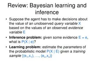
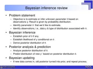
Bayesian inference review • Problem statement • Objective is to estimate or infer unknown parameter q based on observations y. Result is given by probability distribution. • Identify parameter q that we’d like to estimate. • Identify observations, i.e., data y & type of distribution associated with q. • Bayesian inference • Establish prior of q if any. • Establish likelihood of y conditional on q • Derive posterior distribution of q. • Posterior analysis & prediction • Analyze posterior distribution of q. • Predict distribution of new y~ based on posterior distribution q. • Bayesian updating • If new data comes in, old posterior turned into prior, and repeat process.
Bayesian inference review • Bayesian inference • Establish prior of q if any. • Establish likelihood of y conditional on q • Derive posterior distribution of q. Prior distribution Likelihood function Posterior distribution Observed data
Bayesian inference review • Bayesian Inference of a genetic probability • Unknown parameter q • Observation y and its likelihood • Posterior distribution of q • Bayesian inference of binomial problem • Unknown parameter q • Observation y and its likelihood • Posterior distribution of q
Bayesian inference of normal distribution • Problem statement • Objective is to estimate unknown parameters q of normal distribution based on observations y. • Normal distribution has two parameters: mean m & vars2 (stdevs). • Cases of study • We have observations y that follows normal distribution.Single observation yMultiple observations y = {y1, y2, …} • Estimate mean m with known variance s2 • Estimate variance s2 with known mean m • Estimate both parameters will be addressed later.
Fundamentals of normal distribution by matlab • Normal distribution • Probability density function: normpdf(y,m,s) • Cumulative distribution function: normcdf(y,m,s) • Inverse of CDF: norminv(p,m,s)95% confidence intervals • Random sampling and analysis of datanormrnd[mean(y) std(y)][prctile(y,2.5) prctile(y,97.5)]
Estimating mean with known variance • Case of single data (no prior) • Varainces2 known. Mean q = m is unknown. We have single observation y. • No prior on q. Then q ~ constant or just ignore. • Likelihood of y: • Posterior density: • This means when we don’t have any knowledge on the prior distribution, we just estimate the distribution of the mean being the same as the sample distribution. • Practice • Have only one data y=90 with s=10. We want estimate the unknown mean. • Plot the shape of posterior pdf. Superpose original normal distribution. • Posterior prediction
Estimating mean with known variance • Posterior prediction (no prior) • Rearrange the integrand in terms of q to obtain • Ignore 1st term which becomes after integration. Then • Mean is equal to the posterior mean y.Variance is 2s2 or stdev is √2s. So,
Estimating mean with known variance • Case of single data (conjugate prior) • Likelihood of y • Conjugate priorimplies that q is exponential of a quadratic form. • Posterior densityor • Posterior mean is a weighted average of prior mean m0 and observed ywith weights proportional to (inverse of variance) • If t0→ ∞ then c0 → 0, p(q) is constant over (-∞ , ∞). Then we get m1 = y, t1 = s.
Estimating mean with known variance • Posterior prediction (conjugate prior) • Rearrange integrand in terms of q and ignore the resulting term. Then • Mean is equal to the posterior mean.Variance has two components, inherent variance s2 and variance t12 due to the posterior uncertainty in q. So, • If t0→ ∞ then c0 → 0, m1 = y, t1 = s.
Estimating mean with known variance • Case of multiple data (no prior) • Independent & identically distributed (iid) observations • Posterior density • Posterior distribution of the unknown mean follows norm dist with the mean being the sample mean ȳ and the stdev being the sample stdev /√n • Posterior prediction
Estimating mean with known variance • Practice • Observations are 20 data of norm dist where ȳ 2.9 and stdevs 0.2. • Plot posterior pdf of unknown population mean. • Superpose the original normal distribution, assuming ȳ is the true mean. • Plot cdf of the two together.
Estimating variance with known mean • Case of multiple data (non-informative prior) • In case of no information, the prior is • Sample distribution (observation)where • Posterior distributionThe expression is called • Remark • is identical to
Estimating variance with known mean • Evaluation of posterior pdf • Note that • Let us denote then • Then, by the definition of CDF, one can derive the following relation • If we need pdf value of s2, compute z = nv/ s2, next calculate c2pdf value at z. Then multiply z/s2. • If we need cdf of s2, i.e., P[s2 ≤ c] which is same as P[z ≥ zc] of c2pdf .compute zc = nv/c, next calculate 1- c2cdf value at zc.
Fundamentals of Chi2 distribution by matlab • Chi2 distribution • pdf function: chi2pdf(z,n)let’s plot the function when n=5 using pdf & original expression. • cdf function: chi2cdf(z,n) • random samples generation: chi2rnd(z,n) • Posterior distribution of variance s2 • pdf functioncompute z = nv/ s2, next calculate c2pdf value at z. Then multiply z/s2. • Simulation • Random samples of chi2 distribution and comparison with pdf • Random samples of Posterior distribution and comparison with pdf
Estimating variance with known mean • Practice • 5 samples of normal distribution are given with sample variance 0.04. • Plot posterior pdf of unknown variance conditional on the observation using the analytical expression. • Plot the distribution also using the simulation draw. • Superpose the two in one graph. • Calculate the 95% credible interval, i.e., 2.5% & 97.5% percentiles of the distribution.
Homework • Mean with known variance (no prior) n=20 samples of normal distribution with sample mean 2.9 and population stdev 0.2 are given. • write the expression for the posterior distribution of the mean. • plot the posterior distribution of the mean using the pdf function and simulation with N=1e6 respectively. • calculate 2.5%, 97.5% percentiles of the unknown mean from the posterior distribution using the inv function and drawn samples respectively. • Variance with known mean (non-informative prior) n=20 samples of normal distribution with known mean 2.9 and sample stdev 0.2 are given. • write the expression for the posterior distribution of the variance. • plot the posterior distribution of the variance using the pdf function and simulation with N=1e6 respectively. • calculate 2.5%, 97.5% percentiles of the unknown variance from the posterior distribution using the inv function and drawn samples respectively.