Lecture 12: The Constraint Null Space

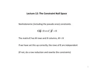
Lecture 12: The Constraint Null Space Nonholonomic (including the pseudo ones) constraints The matrix C has M rows and N columns, M < N If we have set this up correctly, the rows of C are independent (If not, do a row reduction and rewrite the constraints)

Each row is an N row vector The rate of change of q must be perpendicular to all the row vectors There can be K = N – M independent vectors perpendicular to the row vectors of C These vectors form the null space of C Let’s try to say this another way

lives in an N dimensional vector space The rows of C live in the same space The M rows of C form a partial basis in that space must be perpendicular to those basis vectors The vectors that are perpendicular to the rows of C make up the null space there will be K of them, call them s1, s2, etc.

u is a new vector; it is not the u vector we used in the Euler-Lagrange method S is an NxK matrix. Its columns are the basis of the null space. Let’s do a simple example of this before seeing how to use it.

Let’s look at the erect wheel Simple holonomic constraints Generalized coordinates Rolling constraints

The constraint matrix It’s obviously of full rank (rank = 2) There are two vectors in the null space we can work them out on the blackboard and combine them in the S matrix

The rate of change of q becomes If you expand this you will see that u1 and u2 denote the two rotation rates The dimension of u is the true number of degrees of freedom taking the nonholonomic constraints into account.

Let’s move on and see where this can take us. the momentum equations the momentum is a function only of the qs combine in two steps

combine the momentum equation with what we just did momentum equation in terms of u And finally we can get rid of the Lagrange multipliers 0!

Before multiplying by S the free index was i, which runs from 1 to N After multiplying by S, the free index becomes p which runs from 1 to K We have reduced the number of momentum equations to the number of degrees of freedom and gotten rid of the Lagrange multipliers. As usual, it is not as ghastly in practice as it looks in its full generality

We can go back to the erect coin to see how some of this plays out The momentum The velocity equations

The momentum becomes differentiate None of the coordinates appears in the Lagrangian, so the dL/dq term is zero and there are no generalized forces and multiplication by S removes the Lagrange multipliers My equations are simply

Let’s build it expand (continued on the next page)

substitute A lot of trigonometric cancellation leads to the final equations

So, what is the drill? Lagrangian Holonomic constraints Generalized coordinates Nonholonomic constraints Constraint matrix — null space matrix The velocity equations

Hamilton’s momentum equations Eliminate p in favor of u Multiply by S to reduce the number of momentum equations Convert to explicit time dependence for the simulation

What’s new and what’s hard? The idea of the null space is new and finding it can be hard Mathematica can give you a null space, but it may not be what you want I generally work out my own The goal is to devise a null space such that the components of u have a useful interpretation

Multiply C and an arbitrary vector of length N This will give you K conditions from which you can choose K basis vectors Had I done this with the case just reviewed s1 is associated with x, s2 with y, s3 with f and s4 with y I’d like to have one vector for which s3 is unity and one for which s4 is unity

And that’s what I did and that’s why the equations came out so nicely (As it happens, this is the null space that Mathematica gives.)

Let’s look at the 3 x 6 matrix from the two wheel system We can multiply this one out

Do the multiplication and look at the three components of the product We can pick any three and find the others

recall We can take the three spins as fundamental and select bases such that s4 = 1, s5 =0, s6 = 0; s4 = 0, s5 =1, s6 = 0; s4 = 0, s5 =0, s6 = 1

s4 = 1, s5 =0, s6 = 0 and the base vector is

put it all together And the rank of this matrix is obviously three

The advantage of this is that there are fewer equations to deal with The disadvantage is that you do not get the constraint forces (through the Lagrange multipliers) The main consideration is then whether you need the constraint forces If you believe that, whatever they are, the ground will be able to provide them then you may as well adopt the constraint null space method. Let’s look at the two wheel cart using this method

Lecture 12: The Constraint Null Space