Download
1 / 62
620 likes | 776 Vues
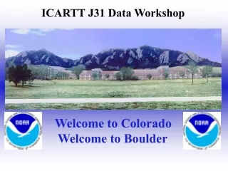
ICARTT J31 Data Workshop March 9, 2005, NOAA Aeronomy Lab, Boulder Particle dispersion modeling with FLEXPART: possibilities for J31 Andreas Stohl Norwegian Institute for Air Research (NILU), Norway Plus GOES 1-km visible satellite products Owen Cooper

E N D
ICARTT J31 Data Workshop March 9, 2005, NOAA Aeronomy Lab, Boulder Particle dispersion modeling with FLEXPART: possibilities for J31 Andreas Stohl Norwegian Institute for Air Research (NILU), Norway Plus GOES 1-km visible satellite products Owen Cooper Cooperative Institute for Research in Environmental Sciences – University of Colorado/ NOAA Aeronomy Laboratory, Boulder
Presentation of the webpagehttp://niwot.al.noaa.gov:8088/icartt_analysiscreated by Andreas Stohl Why does this webpage exist? • For your convenience • To prevent you from using outdated back trajectories for interpreting valuable measurement data
Why are trajectories outdated? Trajectories are not state-of-the-art anymore Trajectories provide no quantitative information Trajectories do not include turbulence and convection Trajectories can be VERY misleading
The new way of doing things right Use a particle dispersion model (FLEXPART) in backward dispersion mode to calculate so-called retroplumes, 20 days back in time. FLEXPART includes turbulence and convection parameterizations and yields a quantitative response function to emissions eventually taken up. Do everything twice using two independent datasets (ECMWF + GFS) to compare results and get a „feeling“ for the uncertainties involved.
What are the input data? GFS analyses: Resolution 1 x 1 degree 26 pressure levels Every 3 hours ECMWF analyses: Resolution 1x1 degree, but 0.36 x 0.36 degree over North America and the Atlantic 60 model levels Every 3 hours
Where are simulations started from? From along the flight tracks: Every time the aircraft changes location by more than 0.2 degree latitude or longitude, or changes altitude by 50 m below 300 m (400 m above 3000 m, 100 m in between). 40.000 particles are released from a small 4-D box (space + time) covering the sampled volume (i.e., a 1-D time box for surface stations). For a given flight, about 200-500 boxes are created