Download
1 / 24
270 likes | 569 Vues
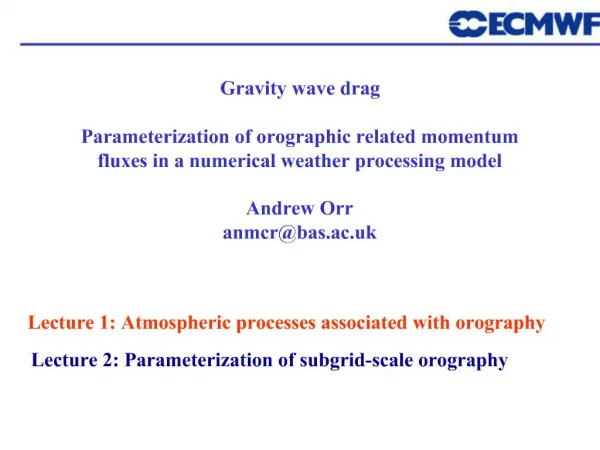
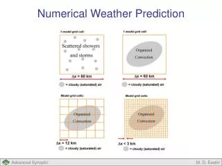
Parametrization of orographic processes in numerical weather processing Andrew Orr andrew.orr@ecmwf.int. Lecture 1: Effects of orography Lecture 2: Sub-grid scale orographic parameterization. History of orography parameterization.

E N D
Parametrization of orographic processes in numerical weather processing Andrew Orr andrew.orr@ecmwf.int Lecture 1: Effects of orography Lecture 2: Sub-grid scale orographic parameterization
History of orography parameterization • Pioneering of studies on linear 2d gravity waves (e.g. Queney, 1948) • Gravity wave drag recognised as important sink of atmospheric momentum (e.g. Eliassen and Palm, 1961) • Observational and modelling studies of non-linear waves (e.g. Lilly, 1978) • Modelling of 3d nonlinear waves • Development of envelope orography (not satisfactory technique for representation of large-scale flow blocking) • Alleviation of systematic westerly bias in numerical weather prediction models through gravity wave drag (GWD) parameterization (Palmer et al. 1986) • High-resolution numerical modelling • Alleviation of inadequate representation of low-level drag through ‘blocked flow’ drag parameterization (Lott and Miller 1997). This is the ECMWF orography parameterization scheme.
Alleviation of systematic westerly bias Mean January sea level pressure (mb) for years 1984 to 1986 (from Palmer et al. 1986) Icelandic/Aleutian lows are too deep Siberian high too weak and too far south Flow too zonal Azores anticyclone too far east Without GWD scheme With GWD scheme Analysis
Alleviation of systematic westerly bias Zonal mean cross-sections of zonal wind (ms-1) and temperature (K, dashed lines) for January 1984 and (a) without GWD scheme and (b) analysis (from Palmer et al 1986) Without GWD scheme temperature too low flow is too strong less impact in southern-hemisphere Analysis
Alleviation of systematic westerly bias Zonal cross-sections of the differences in (a) zonal wind (ms-1) and (b) temperature (K) slowing of winds in stratosphere and upper troposphere poleward induced meridional flow descent over pole leads to warming Parameterisation of gravity wave drag decelerated the predominately westerly flow
High-resolution numerical modelling No GWD scheme large underestimation of drag Sensitivity of pressure drag and momentum fluxes due to the Alps to horizontal resolution From Clark and Miller 1991
Specification of sub-grid orography h: mean topographic height at each gridpoint * * - * * x From Baines and Palmer (1990) h: topographic height above sea level (from global 1km data set) At each gridpoint sub-grid orography represented by: μ: standard deviation of h (amplitude of sub-grid orography) γ: anisotropy (measure of how elongated sub-grid orography is) θ: angle between x-axis and principal axis (i.e. direction of maximum slope) ψ: angle between low-level wind and principal axis of the topography σ: mean slope (along principal axis) 2μ approximates the physical envelope of the peaks Note source grid is filtered to remove small-scale orographic structures and scales resolved by model – otherwise parameterization may simulate unrelated effects
Specification of sub-grid orography Calculate topographic gradient correlation tensor Diagonalise Direction of maximum mean-square gradient at an angle θ to the x-axis
Specification of sub-grid orography Change coordinates (orientated along principal axis) Anisotropy defined as (1:circular; 0: ridge) Slope (i.e. mean-square gradient along the principal axis) If the low-level wind is directed at an angle φ to the x-axis, then the angle ψ is given by: (ψ=0 flow normal to obstacle; ψ=π/2 flow parallel to obstacle)
Resolution sensitivity of sub-grid fields ERA40~120km T511~40km T799~25km
Sub-grid scale orographic parameterisation heff zblk h hz/zblk Gravity wave drag • Compute surface pressure drag exerted on subgrid-scale orography • Compute vertical distribution of wave stress accompanying the surface value Scheme used for: ECMWF (Lott and Miller 1997), UK Met UM, HIRLAM, etc Blocked flow drag • Compute depth of blocked layer • Compute drag at each model level for z < zblk
Evaluation of blocking height Characterise incident (low-level) flow passing over the mountain top by ρH, UH, NH (averaged between μ and 2μ) Define non-dimensional mountain height Hn= hNH/UH In ECMWF model assume h=3μ Blocking height zblk satisfies: Where Hncrit≈1 tunes the depth of the blocked layer (uses wind speed Up calculated by resolving the wind U in the direction of UH)
Evaluation of blocked-flow drag Assume sub-grid scale orography has elliptical shape See Lott and Miller 1997 For z<zblk flow streamlines divide around mountain. Drag exerted by the obstacle on the flow at these levels can be written as l(z): horizontal width of the obstacle as seen by the flow at an upstream height z (assumes each layer below zblk is raised by a factor H/zblk, i.e. reduction of obstacle width) r: aspect ratio of the obstacle as seen by the incident flow Cd (~1): form drag coefficient (proportional to ψ) B,C: constants Summing over number of consecutive ridges in a grid point gives the drag This equation is applied quasi-implicitly level by level below zblk
Evaluation of gravity wave surface stress Consider again an elliptical mountain Gravity wave stress can be written as (Phillips 1984) G (~1): constant (tunes amplitude of waves) Typically L2/4ab ellipsoidal hills inside a grid point. Summing all forces we find the stress per unit area (using a=μ/σ)
Evaluation of stress profile :amplitude of wave :mean Richardson number Gravity wave breaking only active above zblk (i.e. λ=λs for 0<z< zblk) Above zblk stress constant until waves break (i.e. convective overturning) This occurs when the local Richardson number Rimin < Ricrit(=0.25), i.e. saturation hypothesis (Lindzen 1981) Values of the wave stress are defined progressively from the top of the blocked layer upwards
Evaluation of stress profile Calculate Ri at next level Calculate Rimin Height Set λ=λs and Rimin=0.25 at model level representing top of blocked layer Assume stress at any level Uk-3,Tk-3 Set λk-1=λk to estimate δh using k-2 Repeat Uk-2,Tk-2 k-1 If Rimin<Ricrit Uk-1,Tk-1 zk=zblk; λk= λs • set Rimin=Ricrit • estimate h=hsat • estimate = sat • go to next level If Rimin>=Ricrit • estimate h • set k-1= k • go to next level z=0; λ= λs
Gravity wave stress profile U Deceleration Wave breaking 10km Wave breaking Weak winds at low-level can result in low-level wave breaking. Corresponding drag distributed linearly over a depth Δz (above the blocked flow) Note, trapped lee waves not represented in Lott and Miller scheme. However, accounted for in UK Met Office UM model (see Gregory et al. 1998)
Drag contributions From Lott and Miller 1997 T213 forecasts: ECMWF model with mean orography and the subgrid scale orographic drag scheme. Explicit model pressure drag and parameterized mountain drag during PYREX. Strong interaction/compensation between drag contributions
Parameterized surface stresses From ECMWF T511 operational model
Sensitivity of resolved orographic drag to model resolution parameterization still required at high-resolution Strong flow: short-scale trapped lee waves produce significant fraction of drag (Georgelin and Lott, 2001 drag converging Weak flow: most drag produced by flow splitting From Smith et al. 2006
Orographic form drag due to scales <5000m Effective roughness concept (Taylor et al. 1989) Enhancement of roughness length above its vegetative value in areas of orography Disadvantages: Can reach 100’s of meters Roughness lengths for heat and moisture have to be reduced New scheme: Directly parameterises TOFD and distributes it vertically (Beljaars et al. 2004) Vegetative roughness treated independently Requires filtering of orography field to have clear separation of horizontal scales Spectrum of orography represented by piecewise empirical power law Integrates over the spectral orography to represent all relevant scales Wind forcing level of the drag scheme depends on horizontal scale of orography
Enhancement of convection by orography: Simulation of mid-afternoon precipitation maximum
July 2003 mean operational T511 cross-sections of wind (m/s) and specific humidity (g/kg) afternoon morning evening night
References • Baines, P. G., and T. N. Palmer, 1990: Rationale for a new physically based parameterization of sub-grid scale orographic effects. Tech Memo. 169. European Centre for Medium-Range Weather Forecasts. • Beljaars, A. C. M., A. R. Brown, N. Wood, 2004: A new parameterization of turbulent orographic form drag. Quart. J. R. Met. Soc., 130, 1327-1347. • Clark, T. L., and M. J. Miller, 1991: Pressure drag and momentum fluxes due to the Alps. II: Representation in large scale models. Quart. J. R. Met. Soc., 117, 527-552. • Eliassen, A. and E., Palm, 1961: On the transfer of energy in stationary mountain waves, Geofys. Publ., 22, 1-23. • Georgelin, M. and F. Lott, 2001: On the transfer of momentum by trapped lee-waves. Case of the IOP3 of PYREX. J. Atmos. Sci., 58, 3563-3580. • Gregory, D., G. J. Shutts, and J. R. Mitchell, 1998: A new gravity-wave-drag scheme incorporating anisotropic orography and low-level wave breaking: Impact upon the climate of the UK Meteorological Office Unified Model. Quart. J. Roy. Met. Soc., 125, 463-493. • Lilly. D. K., 1978: A severe downslope windstorm and aircraft turbulence event induced by a mountain wave, J. Atmos. Sci., 35, 59-77. • Lindzen, R. S., 1981: Turbulence and stress due to gravity wave and tidal breakdown. J. Geophys. Res., 86, 9707-9714. • Lott, F. and M. J. Miller, 1997: A new subgrid-scale drag parameterization: Its formulation and testing, Quart. J. R. Met. Soc., 123, 101-127. • Queney, P., 1948: The problem of airflow over mountains. A summary of theoretical studies, Bull. Amer. Meteor. Soc., 29, 16-26. • Palmer, T. N., G. J. Shutts, and R. Swinbank, 1986: Alleviation of a systematic westerly bias in general circulation and numerical weather prediction models through an orographic gravity wave drag parameterization, Quart. J. R. Met. Soc., 112, 1001-1039. • Phillips, D. S., 1984: Analytical surface pressure and drag for linear hydrostatic flow over three-dimensional elliptical mountains. J. Atmos. Sci., 41, 1073-1084. • Smith, S., J. Doyle., A. Brown, and S. Webster, 2006: Sensitivity of resolved mountain drag to model resolution for MAP case studies. Submitted to Quart. J. R. Met. Soc.. • Taylor, P. A., R. I. Sykes, and P. J. Mason, 1989: On the parameterization of drag over small scale topography in neutrally-stratified boundary-layer flow. Boundary layer Meteorol., 48, 408-422.