4. MEASUREMENT ERRORS
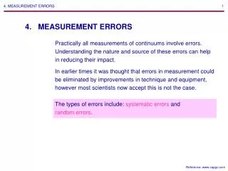
The types of errors include: systematic errors and random errors . 4. MEASUREMENT ERRORS. 4. MEASUREMENT ERRORS. Practically all measurements of continuums involve errors. Understanding the nature and source of these errors can help in reducing their impact.

4. MEASUREMENT ERRORS
E N D
Presentation Transcript
The types of errors include: systematic errors and random errors. 4. MEASUREMENT ERRORS 4. MEASUREMENT ERRORS Practically all measurements of continuums involve errors. Understanding the nature and source of these errors can help in reducing their impact. In earlier times it was thought that errors in measurement could be eliminated by improvements in technique and equipment, however most scientists now accept this is not the case. Reference: www.capgo.com
NB: Systematic errors may change with time, so it is important that sufficient reference data be collected to allow the systematic errors to be quantified. 4. MEASUREMENT ERRORS. 4.1. Systematic errors 4.1. Systematic errors Systematic error are deterministic; they may be predicted and hence eventually removed from data. Systematic errors may be traced by a careful examination of the measurement path: from measurement object, via the measurement system to the observer. Another way to reveal a systematic error is to use the repetition method of measurements. References: www.capgo.com, [1]
4. MEASUREMENT ERRORS. 4.1. Systematic errors Example: Measurement of the voltage source value Temperature sensor Measurement system Rs VS Rin Vin VS Vin VS = a·Vin Rin+RS a = Rin
4. MEASUREMENT ERRORS. 4.2. Random errors. 4.2.1. Uncertainty and inaccuracy 4.2. Random errors 4.2.1. Uncertainty and inaccuracy Random error vary unpredictably for every successive measurement of the same physical quantity, made with the same equipment under the same conditions. We cannot correct random errors, since we have no insight into their cause and since they result in random (non-predictable) variations in the measurement result. When dealing with random errors we can only speak of the probability of an error of a given magnitude. Reference: [1]
NB: Random errors are described in probabilistic terms, while systematic errors are described in deterministic terms. Unfortunately, this deterministic character makes it more difficult to detect systematic errors. 4. MEASUREMENT ERRORS. 4.2. Random errors. 4.2.1. Uncertainty and inaccuracy Reference: [1]
f(x) Mean measurement result 2s Bending point True value 6s (0.14%) (0.14%) Measurements Systematic error Uncertainty Inaccuracy Measurements Amplitude, 0-p rms Maximum random error t 4. MEASUREMENT ERRORS. 4.2. Random errors. 4.2.1. Uncertainty and inaccuracy Example: Random and systematic errors
The upper (most pessimistic) limit of the error interval for any shape of the probability density function is given by the inequality of Chebyshev-Bienaymé: 1 P{x - x ks} , k2 where k is so-called crest* factor (k0). This inequality accretes that the probability deviations that exceed ksis not greater than one over the square of the crest factor. *Crest stands here for ‘peak’. 4. MEASUREMENT ERRORS. 4.2. Random errors. 4.2.2. Crest factor 4.2.2. Crest factor One can define the ‘maximum possible error’ for 100% of the measurements only for systematic errors. For random errors, an maximum random error (error interval) is defined, which is a function of the ‘probability of excess deviations’. Reference: [1]
k2s2 P{x - x ks} k2s2 + x-ks + f(x)dx f(x)dx x+ks - x-ks + 1 = k2s2f(x)dx + k2s2f(x)dx k2s2 - x+ks xx-ks (x-x)2 k2s2 xx+ks (x-x)2 k2s2 x-ks + 1 (x-x)2f(x)dx + (x-x)2f(x)dx k2s2 - x+ks s2 x-ks x+ks + 1 (x-x)2f(x)dx + (x-x)2f(x)dx + (x-x)2f(x)dx k2s2 - x-ks x+ks 1 . k2 4. MEASUREMENT ERRORS. 4.2. Random errors. 4.2.2. Crest factor Proof:
4. MEASUREMENT ERRORS. 4.2. Random errors. 4.2.2. Crest factor Note that the Chebyshev-Bienaymé inequality can be derived from the Chebyshev inequality which can be derived from the Markov inequality s2 P{x - x a} , a2 x P{ x a} . a x0
Tchebyshev (most pessimistic) limit any pdf 4. MEASUREMENT ERRORS. 4.2. Random errors. 4.2.2. Crest factor Illustration: Probability of excess deviations Normal pdf 100 10-1 10-2 10-3 Probability of excess deviations 10-4 10-5 10-6 0 1 2 3 4 5 Crest factor, k
We will discuss this analysis first for systematic errors and then for random errors. 4.3.1. Systematic errors Let us define the absolute error as the difference between the measured and true values of a physical quantity, Da a -a0 , 4. MEASUREMENT ERRORS. 4.3. Error propagation 4.3. Error sensitivity analysis The sensitivity of a function to the errors in arguments is called error sensitivity analysis or error propagation analysis. Reference: [1]
4. MEASUREMENT ERRORS. 4.3. Error propagation. 4.3.2. Systematic errors and the relative error as: Da a - a0 da = . a0 a0 If the final result x of a series of measurements is given by: x = f(a,b,c,…), where a, b, c ,… are independent, individually measured physical quantities, then the absolute error of x is: Dx = f(a,b,c,…)-f(a0,b0,c0,…). Reference: [1]
f(a,b,c,…) Dx = Da a 4. MEASUREMENT ERRORS. 4.3. Error propagation. 4.3.2. Systematic errors With a Taylor expansion of the first term, this can also be written as: in which all higher-order terms have been neglected. This is permitted provided that the absolute errors of the arguments are small and the curvature of f(a,b,c,…) at the point (a,b,c,…) is small. f(a,b,c,…) + Db + …, b (a0,b0,c0,…) (a0,b0,c0,…) Reference: [1]
4. MEASUREMENT ERRORS. 4.3. Error propagation. 4.3.2. Systematic errors One never knows the actual value of Da,Db,Dc,… . Usually the individual measurements are given as a± Damax, b± Dbmax,… , in which Damax,Dbmax are the maximum possible errors. In this case f(a,b,c,…) f(a,b,c,…) Dxmax = Damax + Dbmax + … . a b (a0,b0,c0,…) (a0,b0,c0,…) Reference: [1]
4. MEASUREMENT ERRORS. 4.3. Error propagation. 4.3.2. Systematic errors Defining the sensitivity factors: f S xa , … , a (a0,b0,c0,…) this becomes: Dxmax S xaDamax + S xb Dbmax + … . Reference: [1]
4. MEASUREMENT ERRORS. 4.3. Error propagation. 4.3.2. Systematic errors This expression can be rewritten to obtain the maximal relative error: Dxmax fa Damax fb Dbmax dxmax = + + … . a f0 a b f0 b x0 Defining the relative sensitivity factors: fa df f/f0 sxa = = , … , a f0 da a/a this becomes: dxmax sxadamax + sxb dbmax + … . Reference: [1]
2da 6da da b = a2 x = b3 2. sxa = sxb sba 2da da x1 = a2 da 3. sx1 x2a = sx1a+ sx2a + -da da x2 = -a 4. MEASUREMENT ERRORS. 4.3. Error propagation. 4.3.2. Systematic errors Illustration: The rules that simplify the error sensitivity analysis da 2da m n x = a2 1. sxa = sxa n m
f f f a b c dx = da + db + dc + …. (a,b,c,…) (a,b,c,…) (a,b,c,…) 4. MEASUREMENT ERRORS. 4.3. Error propagation. 4.3.2. Random errors 4.3.2. Random errors If the final result x of a series of measurements is given by: x = f(a,b,c,…), where a, b, c, … are independent, individually measured physical quantities, then the absolute error of x is: Again, we have neglected the higher order terms of the Taylor expansion. Reference: [1]
(a,b,c,…) (a,b,c,…) 4. MEASUREMENT ERRORS. 4.3. Error propagation. 4.3.2. Random errors Since dx= x-x, f 2 f f s2 = (dx)2 = da + db + dc + … . c a b 2 2 f f f f = (da)2 + (db)2 + …+ da db + … a b a b squares cross products (=0) 2 2 f f = (da)2 + (db)2 + … . a b Reference: [1]
2 2 2 f f f sx2 = sa2 + sb2 + sc2 + … a b c x = f(a,b,c,…) (a,b,c,…) (a,b,c,…) (a,b,c,…) NB: In the above derivation, the shape of the pdf of the individual measurements a, b, c, … does not matter. 4. MEASUREMENT ERRORS. 4.3. Error propagation. 4.3.2. Random errors Considering that (da)2 sa2 …, the expression for sx2 can be written as (Gauss’ error propagation rule): Reference: [1]
n 1 n x = ai : i = 1 or for the standard deviation of the end result: Thanks to averaging, the measurement uncertainty decreases with the square root of the number of measurements. 1 n sx = sa . 4. MEASUREMENT ERRORS. 4.3. Error propagation. 4.3.2. Random errors Example A: Let us apply Gauss’ error propagation rule to the case of averaging in which 1 n 1 n2 x = a . sx2= n sa2 = sa2,
Due to integration, the measurement uncertainty increases with the square root of the number of measurements. 4. MEASUREMENT ERRORS. 4.3. Error propagation. 4.3.2. Random errors Example B: Let us apply Gauss’ error propagation rule to the case of integration in which n x = ai : i = 1 x = a . sx2= nsa2 , i = or for the standard deviation of the end result: sx = n sa .
1 n sx = sa 4. MEASUREMENT ERRORS. 4.3. Error propagation. 4.3.2. Random errors Illustration: Noise averaging and integration Input Output Gaussian white noise Averaging(10) and integration Averaging Integration sx = n sa
4. MEASUREMENT ERRORS. 4.3. Error propagation. 4.3.2. Random errors Illustration: LabView simulation
Next lecture Next lecture: