Download
1 / 42
420 likes | 706 Vues
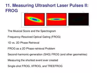
11. Measuring Ultrashort Laser Pulses II: FROG. The Musical Score and the Spectrogram Frequency-Resolved Optical Gating (FROG) 1D vs. 2D Phase Retrieval FROG as a 2D Phase-retrieval Problem Second-harmonic-generation (SHG) FROG (and other geometries)

E N D
11. Measuring Ultrashort Laser Pulses II: FROG The Musical Score and the Spectrogram Frequency-Resolved Optical Gating (FROG) 1D vs. 2D Phase Retrieval FROG as a 2D Phase-retrieval Problem Second-harmonic-generation (SHG) FROG (and other geometries) Measuring the shortest event ever created Single-shot FROG, XFROG, and TREEFROG
Autocorrelation and related techniques yield little information about the pulse. Perhaps it’s time to ask how researchers in other fields deal with their waveforms… Consider, for example, acoustic waveforms.
Most people think of acoustic waves in terms of a musical score. It’s a plot of frequency vs. time, with information on top about the intensity. The musical score lives in the “time-frequency domain.”
Spectrogram If E(t) is the waveform of interest, its spectrogram is: where g(t-t) is a variable-delay gate function and t is the delay. Without g(t-t), SpE(w,) would simply be the spectrum.
Spectrograms for Linearly Chirped Pulses Frequency Time Frequency Delay
Properties of the Spectrogram = The Intensity. No phase information! Algorithms exist to retrieve E(t) from its spectrogram. The spectrogram essentially uniquely determines the waveform intensity, I(t), and phase, (t). There are a few ambiguities, but they are “trivial.” The gate need not be—and should not be—significantly shorter than E(t). Suppose we use a delta-function gate pulse: The spectrogram resolves the dilemma! It doesn’t need the shorter event! It temporally resolves the slow components and spectrally resolves the fast components.
Frequency-Resolved Optical Gating (FROG) “Polarization-Gate” Geometry Spectro- meter Trebino, et al., Rev. Sci. Instr., 68, 3277 (1997). Kane and Trebino, Opt. Lett., 18, 823 (1993).
FROG Traces for Linearly Chirped Pulses Frequency Time Frequency Delay
FROG Traces for More Complex Pulses Intensity Frequency Time Frequency Frequency Delay Delay
The FROG trace is a spectrogram of E(t). Substituting for Esig(t,) in the expression for the FROG trace: Esig(t,) E(t) |E(t–)|2 yields: g(t–)|E(t–)|2 where: Unfortunately, spectrogram inversion algorithms require that we know the gate function.
Instead, consider FROG as a two-dimensional phase-retrieval problem. The input pulse, E(t), is easily obtained from Esig(t,W): E(t)Esig(t,) If Esig(t,), is the 1D Fourier transform with respect to delay t of some new signal field, Esig(t,W), then: and So we must invert this integral equation and solve for Esig(t,W). This integral-inversion problem is the 2D phase-retrieval problem, for which the solution exists and is unique. And simple algorithms exist for finding it. Stark, Image Recovery, Academic Press, 1987.
1D vs. 2D Phase Retrieval We assume that E(t) and E(x,y) are of finite extent. 1D Phase Retrieval: Suppose we measure S(w) and desire E(t), where: Given S(w), there are infinitely many solutions for E(t). We lack the spectral phase. 2D Phase Retrieval: Suppose we measure S(kx,ky) and desire E(x,y): Stark, Image Recovery, Academic Press, 1987. Given S(kx,ky), there is essentially one solution for E(x,y)!!! It turns out that it’s possible to retrieve the 2D spectral phase! . These results are related to the Fundamental Theorem of Algebra.
Phase Retrieval and the Fundamental Theorem of Algebra The Fundamental Theorem of Algebra states that all polynomials can be factored: fN-1 zN-1 + fN-2 zN-2 + … + f1 z + f0 = fN-1 (z–z1 )(z–z2 ) … (z–zN–1) The Fundamental Theorem of Algebra fails for polynomials of two variables. Only a set of measure zero can be factored. fN-1,M-1 yN-1 zM-1 + fN-1,M-2 yN-1zM-2 + … + f0,0 = ? Why does this matter? The existence of the 1D Fundamental Theorem of Algebra implies that 1D phase retrieval is impossible. The non-existence of the 2D Fundamental Theorem of Algebra implies that 2D phase retrieval is possible.
Phase Retrieval & the Fund Thm of Algebra 2 1D Phase Retrieval and the Fundamental Theorem of Algebra The Fourier transform {F0 , … , FN-1} of a discrete 1D data set, { f0 , …, fN-1}, is: where z = e–ik polynomial! The Fundamental Theorem of Algebra states that any polynomial, fN-1zN-1 + … + f0 , can be factored to yield: fN-1 (z–z1 )(z–z2 ) … (z–zN–1) So the magnitude of the Fourier transform of our data can be written: |Fk| = | fN-1 (z–z1 )(z–z2 ) … (z–zN–1) | where z = e–ik Complex conjugation of any factor(s) leaves the magnitude unchanged, but changes the phase, yielding an ambiguity! So 1D phase retrieval is impossible!
Phase Retrieval & the Fund Thm of Algebra 2 2D Phase Retrieval and the Fundamental Theorem of Algebra The Fourier transform {F0,0 , … , FN-1,N-1} of a discrete 2D data set, { f0.0 , …, fN-1,N-1}, is: where y = e–ik and z = e–iq Polynomial of 2 variables! But we cannot factor polynomials of two variables. So we can only complex conjugate the entire expression (yielding a trivial ambiguity). Only a set of polynomials of measure zero can be factored. So 2D phase retrieval is possible! And the ambiguities are very sparse.
Generalized Projections Esig(t,) E(t) |E(t–)|2 Esig(t,)
Algorithm such that Find Esig(t,) and is as close as possible to Esig(t,) E(t) DeLong and Trebino, Opt. Lett., 19, 2152 (1994) Code is available commercially from Femtosoft Technologies.
Applying the Signal Field Constraint We must find such that and is as close as possible to Esig(t,). The way to do this is to find the field, E(t), that minimizes: Once we find the E(t) that minimizes Z, we write the new signal field as: DeLong and Trebino, Opt. Lett., 19, 2152 (1994) This is the new signal field in the iteration.
Second-Harmonic-Generation FROG Kane and Trebino, JQE, 29, 571 (1993). DeLong and Trebino, JOSA B, 11, 2206 (1994). Second-harmonic generation (SHG) is the strongest NLO effect.
SHG FROG traces are symmetrical with respect to delay. Frequency Time Frequency Delay
SHG FROG traces for complex pulses Intensity Frequency Time Frequency Frequency Delay Delay
SHG FROG Measurements of a Free-Electron Laser Richman, et al., Opt. Lett., 22, 721 (1997). 5 5 4 4 3 3 Spectral Phase (rad) Intensity Spectral Intensity Phase (rad) 2 2 1 1 0 0 -4 -2 0 2 4 5076 5112 5148 Time (ps) Wavelength (nm) SHG FROG works very well, even in the mid-IR and for difficult sources.
Shortest pulse vs. year Plot prepared in 1994 (by Erich Ippen, MIT) reflecting the state of affairs at that time. Shortest pulse length Year
The measured pulse spectrum had two humps, and the measured autocorrelation had wings. Two different theories emerged, and both agreed with the data. From Harvey et. al, Opt. Lett., v. 19, p. 972 (1994) From Christov et. al, Opt. Lett., v. 19, p. 1465 (1994) 10-fs spectra and autocorrs Data courtesy of Kapteyn and Murnane, WSU Despite different predictions for the pulse shape, both theories were consistent with the data.
FROG distinguishes between the theories. Taft, et al., J. Special Topics in Quant. Electron., 3, 575 (1996).
SHG FROG Measurements of a 4.5-fs Pulse! Baltuska, Pshenichnikov, and Weirsma, J. Quant. Electron., 35, 459 (1999).
Using SHG FROG to study materials Using SHG FROG to study materials The evolution of a pulse propagating through a fiber Delay Frequency Frequency Fatemi and coworkers, Optics Express 2002
Generalizing FROG to arbitrary nonlinear-optical interactions Pulse retrieval remains equivalent to the 2D phase-retrieval problem. Many interactions have been used, e.g., polarization rotation in a fiber.
FROG geometries: Pros and Cons Second- harmonic generation most sensitive; most accurate Third- harmonic generation tightly focused beams useful for UV & transient-grating experiments Transient- grating simple, intuitive, best scheme for amplified pulses Polarization- gate Self- diffraction useful for UV
Generalized Projections with an Arbitrary Medium Response DeLong, et al., Opt. Lett. 20, 486 (1995).
Single-shot FROG Crossing beams at a large angle produces a range of delays across the nonlinear-optical medium and maps delay onto transverse position.
Single-Shot Polarization-Gate FROG Kane and Trebino, Opt. Lett., 18, 823 (1993).
FROG allows a very simple imaging spectrometer. We can use the focus of the beam in the nonlinear medium as the entrance slit for a home-made imaging spectrometer (in multi-shot and single-shot FROG measurements). Signal pulse Collimating Lens Pulses from first half of FROG Grating Nonlinear Medium Imaging Lens Camera or Linear Detector Array This eliminates the need for a bulky expensive spectrometer as well as the need to align the beam through a tiny entrance slit (which would involve three sensitive alignment parameters)!
When a known reference pulse is available:Cross-correlation FROG (XFROG) If a known pulse is available (it need not be shorter), then it can be used to fully measure the unknown pulse. In this case, we perform sum-frequency generation, and measure the spectrum vs. delay. SFG crystal E(t) Camera Spectro- meter Unknown pulse Eg(t–t) Known pulse Lens The XFROG trace (a spectrogram): XFROG completely determines the intensity and phase of the unknown pulse, provided that the gate pulse is not too long or too short. If a reasonable known pulse exists, use XFROG, not FROG. Linden, et al., Opt. Lett., 24, 569 (1999).
XFROG trace XFROG example: Ultrabroadband Continuum Ultrabroadband continuum was created by propagating 1-nJ, 800-nm, 30-fs pulses through 16 cm of Lucent microstructure fiber. The 800-nm pulse was measured with FROG, so it made an ideal known gate pulse. Retrieved intensity and phase Kimmel, Lin, Trebino, Ranka, Windeler, and Stentz, CLEO 2000. This pulse has a time-bandwidth product of ~ 4000, and is the most complex ultrashort pulse ever measured.
TREEFROG Example DeLong, et al., JOSA B, 12, 2463 (1995). TREEFROG is still under active study, and many variations exist. It will be useful in excite-probe spectroscopic measurements, which involve crossing two pulses with variable relative delay at a sample.