19. Theory of Ultrashort Laser Pulse Generation

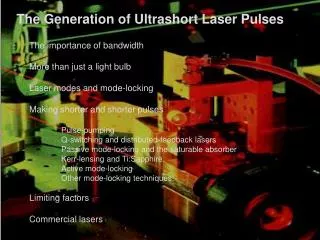
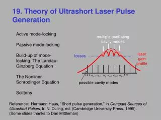
1. multiple oscillating cavity modes laser gain profile losses wq-2 wq-1 wq wq+1 wq+2 wq+3 possible cavity modes 19. Theory of Ultrashort Laser Pulse Generation Active mode-locking Passive mode-locking Build-up of mode-locking: The Landau-Ginzberg Equation The Nonliner Schrodinger Equation Solitons Reference: Hermann Haus, “Short pulse generation,” in Compact Sources of Ultrashort Pulses, Irl N. Duling, ed. (Cambridge University Press, 1995). (Some slides thanks to Dan MIttleman)

2. multiple oscillating cavity modes laser gain profile losses wq-2 wq-1 wq wq+1 wq+2 wq+3 possible cavity modes Mode-locking yields ultrashort pulses. Multiple modes can oscillate simultaneously in a cavity Sum of ten modes with the same relative phase Sum of ten modes w/ random phase

3. Mechanisms for Mode Locking Active Mode Locking Insert something into the laser cavity that modulates the amplitude of the pulse.  mode competition couples each mode to modulation sidebands  eventually, all the modes are coupled and phase-locked Passive Mode Locking Insert something into the laser cavity that favors high intensities.  strong maxima will grow stronger at the expense of weaker ones  eventually, all of the energy is concentrated in one packet

4. modulator transmission cos(wMt) Time wn+wM wn-wM w0 Frequency Active Mode- Locking In the frequency domain, a modulator introduces side-bands. For mode-locking, make sure that wM = mode spacing. This means that: wM = 2p/cavity round-trip time cavity modes Each mode competes for gain with the sidebands of the adjacent modes. Most efficient operation is for phases to lock Result is global phase locking n coupled equations: En En+1, En-1

5. Active mode-locking by amplitude modulation Gain exceeds loss for only a short time during each round trip.

6. wM w The laser modes and gain Lasers have a mode spacing: w0 Let the zeroth mode be at the center of the gain, w0. The nth mode frequency is then: Let an be the amplitude of the nth mode and assume a Lorentzian gain profile, G(n):

7. Notice that this spreads the energy from the nth to the (n+1)st and (n-1)st modes. Including the loss, , we can write this as: An amplitude modulator An amplitude modulator uses the electro-optic or acousto-optic effect to deliberately cause losses at the laser round-trip frequency, wM. A modulator multiplies the laser light (i.e., each mode) by M[1-cos(wMt)] where the superscript indicates the kth round trip.

8. where, in this continuous limit, where: Solve for the steady-state solution In steady state, Also, the finite difference becomes a second derivative when the modes are many and closely spaced: This differential equation has the solution: with the constraints: In practice, the lowest-order mode occurs: A Gaussian!

9. Fourier-transforming to the time domain Recalling that multiplication by -w2 in the frequency domain is just a second derivative in the time domain (and vice versa): which has the solution: This makes sense because Hermite-Gaussians are their own Fourier transforms. The time-domain will prove to be a better domain for modeling passive mode-locking.

10. Fast absorber Slow absorber loss loss gain gain gain > loss gain > loss time time Passive Mode-Locking Saturable gain: • gain saturates during the passage of the pulse • leading edge is selectively amplified Saturable absorption: • absorption saturates during the passage of the pulse • leading edge is selectively eroded

11. Saturable-absorber mode-locking Neglect gain saturation, and model a fast saturable absorber: The transmission through a fast saturable absorber: where: Including this additional loss, l, in the mode-amplitude equation: Lumping the constant loss into l

12. The sech pulse shape In steady state, this equation has the solution: where the conditions on t and A0 are:

13. The Master Equation: Including GVD Expand k to second order in w: After propagating a distance Ld, the amplitude becomes: Ignore the constant phase and vg, and expand the 2nd-order phase: Inverse-Fourier-transforming: where:

14. The Master Equation (continued): Including the Kerr effect The Kerr Effect: so: The master equation (assuming small effects) becomes: (we’re converting a(k) to a(t)) In steady state: This important equation is called the Landau-Ginzberg Equation.

15. Solution to the Master Equation It is: where: The complex exponent yields chirp.

16. The Pulse Length and Chirp Parameter

17. The Spectral Width The spectral width vs. dispersion for various SPM values. A broader spectrum is possible if some positive chirp is acceptable.

18. Stability of solutions The laser will be stable when the gain is less than the loss just before and just after the pulse. Instability for high SPM

19. Intensity Short time (fs) k = 1 k = 2 k = 3 Long time (round trips) (ns) k = 7 Notice that the weak pulses are suppressed, and the strong pulse shortens and is amplified. The Nonlinear Schrodinger Equation First, imagine raster-scanning the pulse vs. time like this: We’ll call the long-time round-trip-number axis “z”.

20. The Nonlinear Schrodinger Equation Recall the master equation: which becomes (when we assume many round trips and let k be z): Neglecting every effect in this equation, except for the Kerr effect and GVD, we have the Nonlinear Schrodinger Equation:

21. The Nonlinear Schrodinger Equation The solution to the nonlinear Shrodinger equation is: where: and Dw is the detuning from w0. Note that d/D < 0, or no solution exists. But note that, despite dispersion, the pulse length and shape do not vary with distance.

22. Solitons and solitary waves A “solitary wave” is a wave that retains its shape, despite dispersion and nonlinearities. A “soliton” is a pulse that can collide with another similar pulse and still retain its shape after the collision, again in the presence of both dispersion and nonlinearities.

23. Collision of two solitons

24. Evolution of a soliton from a square wave

25. Higher-Order Soliton

26. Other Mode-Locking Techniques FM mode-locking produce a phase shift per round trip implementation: electro-optic modulator similar results in terms of steady-state pulse duration Synchronous pumping • gain medium is pumped with a pulsed laser, at a rate of 1 pulse per • round trip • requires an actively mode-locked laser to pump your laser ($$) • requires the two cavity lengths to be accurately matched • useful for converting long AM pulses into short AM pulses • (e.g., 150 psec argon-ion pulses  sub-psec dye laser pulses) Additive-pulse or coupled-cavity mode-locking external cavity which feeds pulses back into main cavity synchronously requires two cavity lengths to be matched can be used to form sub-100-fsec pulses