CDV derivation
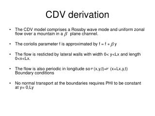
CDV derivation. The CDV model comprises a Rossby wave mode and uniform zonal flow over a mountain in a plane channel. The coriolis parameter f is approximated by f = f + y The flow is resticted by lateral walls with width 0< y<Lx and length 0<x<Lx.

CDV derivation
E N D
Presentation Transcript
CDV derivation • The CDV model comprises a Rossby wave mode and uniform zonal flow over a mountain in a plane channel. • The coriolis parameter f is approximated by f = f + y • The flow is resticted by lateral walls with width 0< y<Lx and length 0<x<Lx. • The flow is also periodic in longitude so (x,y,t)= (x+Lx,y,t) Boundary conditions • No normal transport at the boundaries requires PHI to be constant at y= 0,Ly
CDV Derivation • The equation used in the model is the QGPV equation • To derive the low order spectral model you must expand , , and h(x,y) into orthonormal eigenfunctions of the Leplace operator. • This derivation is very complex. I will show a more general representation by solving Leplace’s equation on a rectangle and introducing the concept of orthogonality.
CDV Derivation • Laplace equation • Break the problem into four problems with each having one homogeneous condition • Separate the variables • Solve x dependent equation and y dependent equation. • Use boundary conditions and orthogonality to find coefficients
CDV derivation • Orthogonality • Whenever it is said that functions are orthogonal over the interval 0<x<L. The term is borrowed from perpendicular vectors because the integral is analogous to a zero dot product
CDV Derivation • The process is similar in the derivation of the CDV model • First you have to non-dimensionalize the QGPV equation.(A1,A2) • Represent h(x,y) and PHI* in terms of sines and cosines(A3), and expand PHI into three orthonormal modes(A4).
CDV derivation • Insert A3 and A4 back into the A1. • This leads to the following equations known as the CDV equations. • The CDV equations are solved to find the equilibrium points
CDV model • As we found from holton, the system has three equilibria point. One unstable and two stable(Show graphic again?) • For arbitrary initial conditions the phase space trajectories always tend to one of the two stable equilibria • This is a drawback of the CDV model because there is no way to transition between the two stable equilibra points.