Download

1 / 54
540 likes | 754 Vues
On bifurcation in counter-flows of viscoelastic fluid. Preliminary work. Mackarov I. Numerical observation of transient phase of viscoelastic fluid counterflows // Rheol. Acta. 2012, Vol. 51, Issue 3, Pp. 279-287 DOI 10.1007/s00397-011-0601-y.

E N D
Preliminary work • Mackarov I. Numerical observation of transient phase ofviscoelasticfluid counterflows // Rheol. Acta. 2012, Vol. 51, Issue 3,Pp. 279-287DOI 10.1007/s00397-011-0601-y. • Mackarov I. Dynamic features of viscoelastic fluid counter flows // Annual Transactions of the Nordic Rheology Society. 2011. Vol. 19. Pp. 71-79.
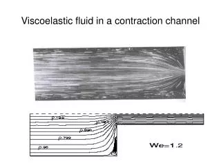
The process of the flow reversal, Re = 0.1, Wi= 4, mesh is675nodes,t=1.7 ÷2.5
The process of the flow reversal, Re= 0.1, Wi = 4, mesh is675nodes,t=1.7 ÷2.5
G.N. Rocha and P.J. Oliveira.Inertial instability in Newtonian cross-slot flow– A comparison againstthe viscoelastic bifurcation.Flow Instabilities and Turbulence in Viscoelastic Fluids, Lorentz Center, July 19-23, 2010, Leiden, Netherlands • R. J. Poole, M. A. Alves, and P. J. Oliveira.Purely Elastic Flow Asymmetries. Phys. Rev. Lett., 99,164503, 2007.
Vicinity of the central point: symmetric case
Symmetry relativeto x, y definesthe most general asymptotic form of velocities: … and stresses:
Substituting this to momentum, continuity, and UCM state equations will give…
Symmetry on x, y involves (21) Therefore, for the rest of the coefficients in solution ,
Pressure: from momentum equation where
Comparison with symmetric numerical solution
Via finite-difference expressions of coefficients in velocities expansions, we get from the numeric solution: A ≈ -0.006B ≈ 0.0032
STRESS: Via finite-difference determination of coefficients in velocities expansions get : Σx= -0.0573α = 0.0286 β = 0.026≈ α “Numerical” stress in the central point : σxx= -0.0518
Normal stress distribution in numericone-quadrantsolution (stabilized regime),Re=0.1, Wi=4, the mesh is 2600 nodes
PRESSURE: Via finite-difference values of coefficients in velocities expansions, we get : Px=0.0642 Py=-0.0641 ≈-Px
Vicinity of the central point: asymmetric case
Looking into nature of the flow reversal: analogy with simpler flows • Couette flow • Poiseuille flow
Pressure distributionin the flow with Re = 3andWi= 4at t =3.5, meshis1200nodes, Δt= 5·10-5
Both some features reported before and new details were observed in simulation of counter flows within cross-slots (acceleration phase). • Among the new ones: the pressure and stresses singularities both at the stagnation point and at the walls corner, flow reversal with vortex-like structures. • The flow reverse is shown to result fromthe wave nature of a viscoelastic fluid flow.
Flow picture (UCM model, Re = 0.05, Wi = 4, t=6.2), with exponential lowof the pressure increase (α = 1) the meshis432nodes
Convergence and quality of numerical procedure
Picture of vortices typical fortypical for small Re.UCM model, Re = 0.1, Wi = 4, t=2.6, mesh is1200nodes
The same flow snapshot(UCM model, Re = 0.1, Wi = 4, t=2.6), obtained on a non-elastic meshwith 1200 nodes
Normal stress distribution in the flow with Re = 0.01 andWi=100 at t = 3; UCM model, meshis2700nodes, Δt= 5·10-5
Sequence of normal stress abs. values at the stagnation point. Smaller markers correspond to time step 0.0001, bigger ones are for time step 0.00005
High Weissenberg numbers: Sequence of normal stress abs. values at the stagnation point. Smaller markers correspond to time step 0.0001, bigger ones are for time step 0.00005
Normal stress distribution in the flow with Re = 0.1 andWi =4at t = 3; meshis 450 nodes, Δt= 5·10-5
The process of the flow reversal, Re = 0.1, Wi= 4, mesh is675nodes,t=1.7 ÷2.5
A flow snapshot from S. J. Haward et. al., The rheology of polymer solution elastic strands in extensional flow, Rheol Acta (2010) 49:781-788