Numerical simulation of Fluid flows
450 likes | 484 Vues
Introduction<br>Fluids and flows<br>Numerical Methods<br>Mathematical description of flows<br>Finite volume method<br>Turbulent flows<br>Example with CFX<br>

Numerical simulation of Fluid flows
E N D
Presentation Transcript
Numericalsimulation of fluid flows Rushi Kumar B Department of Mathematics School of Advanced Sciences Vellore Institute of Technology, Vellore
Overview • Introduction • Fluids and flows • Numerical Methods • Mathematical description of flows • Finite volume method • Turbulent flows • Example with CFX
Introduction In the past, two approaches in science: • Theoretical • Experimental Computer Numerical simulation Computational Fluid Dynamics (CFD) Expensive experiments are being replaced by numerical simulations : - cheaper and faster - simulation of phenomena that can not be experimentally reproduced (weather, ocean, ...)
Fluids and flows Liquids and gases obey the same laws of motion Most important properties: density and viscosity A flow is incompressible if density is constant. liquids are incompressible and gases if Mach number of the flow < 0.3 Viscosity: measure of resistance to shear deformation
Fluids and flows (2) Far from solid walls, effects of viscosity neglected inviscid (Euler) flow in a small region at the wall boundary layer Important parameter: Reynolds number ratio of inertial forces to friction forces • creeping flow • laminar flow • turbulent flow
Fluids and flows (3) • Lagrangian description follows a fluid particle as it moves through the space • Eulerian description focus on a fixed point in space and observes fluid particles as they pass Both points of view related by the transport theorem
Numerical Methods Navier-Stokes equations analytically solvable only in special cases approximate the solution numerically use a discretization method to approximate the differential equations by a system of algebraic equations which can be solved on a computer • Finite Difference Method (FDM) • Finite Volume Method (FVM) • Finite Element Method (FEM)
Numerical methods, grids Grids • Structured grid • all nodes have the same number of elements around it • only for simple domains • Unstructured grid • for all geometries • irregular data structure • Block-structured grid
Numerical methods, properties Consistency Truncation error : difference between discrete eq and the exact one • Truncation error becomes zero when the mesh is refined. • Method order n if the truncation error is proportional to or Stability • Errors are not magnified • Bounded numerical solution
Numerical methods, properties (2) Convergence • Discrete solution tends to the exact one as the grid spacing tends to zero. • Lax equivalence theorem (for linear problems): Consistency + Stability = Convergence • For non-linear problems: repeat the calculations in successively refined grids to check if the solution converges to a grid-independent solution.
Mathematical description of flows • Conservation of mass • Conservation of momentum • Conservation of energy of a fluid particle (Lagrangian point of view). For computations is better Eulerian (fluid control volume) Transport theorem volume of fluid that moves with the flow
Fluid element infinitesimal fluid element 6 faces: North, South, East, West, Top, Bottom Systematic account of changes in the mass, momentum and energy of the fluid element due to flow across the boundaries and the sources inside the element fluid flow equations
Transport equation General conservative form of all fluid flow equations for the variable Transport equation for the property
Transport equation (2) Integration of transport equation over a CV Using Gauss divergence theorem,
Boundary conditions • Wall : no fluid penetrates the boundary • No-slip, fluid is at rest at the wall • Free-slip, no friction with the wall • Inflow (inlet): convective flux prescribed • Outflow (outlet): convective flux independent of coordinate normal to the boundary • Symmetry
Finite Volume Method Starting point: integral form of the transport eq (steady) control volume CV
Approximation of volume integrals • simplest approximation: • exact if q constant or linear • Interpolation using values of q at more points • Assumption q bilinear
Approximation of surface integrals Net flux through CV boundary is sum of integrals over the faces • velocity field and density are assumed known • is the only unknown • we consider the east face
Approximation of surface integrals (2) Values of f are not known at cell faces interpolation
Interpolation • we need to interpolate f • the only unknown in f is Different methods to approximate and its normal derivative: • Upwind Differencing Scheme (UDS) • Central Differencing Scheme (CDS) • Quadratic Upwind Interpolation (QUICK)
Interpolation (2) Upwind Differencing Scheme (UDS) • Approximation by its value the node upstream of ‘e’ • first order • unconditionally stable (no oscillations) • numerically diffusive
Interpolation (3) Central Differencing Scheme (CDS) • Linear interpolation between nearest nodes • second order scheme • may produce oscillatory solutions
Interpolation (4) Quadratic Upwind Interpolation (QUICK) Interpolation through a parabola: three points necessary P, E and point in upstream side • g coefficients in terms of nodal coordinates • third order
Linear equation system • one algebraic equation at each control volume • matrix A sparse • Two types of solvers: • Direct methods • Indirect or iterative methods
Linear eq system, direct methods Direct methods • Gauss elimination • LU decomposition • Tridiagonal Matrix Algorithm (TDMA) - number of operations for a NxN system is - necessary to store all the coefficients
Linear eq system, iterative methods Iterative methods • Jacobi method • Gauss-Seidel method • Successive Over-Relaxation (SOR) • Conjugate Gradient Method (CG) • Multigrid methods - repeated application of a simple algorithm - not possible to guarantee convergence - only non-zero coefficients need to be stored
Time discretization For unsteady flows, initial value problem • f discretized using finite volume method • time integration like in ordinary differential equations right hand side integral evaluated numerically
Time discretization (3) Types of time integration methods • Explicit, values at time n+1 computed from values at time n Advantages: - direct computation without solving system of eq - few number of operations per time step Disadvantage: strong conditions on time step for stability • Implicit, values at time n+1 computed from the unknown values at time n+1 Advantage: larger time steps possible, always stable Disadv: - every time step requires solution of a eq system - more number of operations
Coupling of pressure and velocity • Up to now we assumed velocity (and density) is known • Momentum eq from transport eq replacing by u, v, w
Coupling of pressure and velocity (2) • Non-linear convective terms • Three equations are coupled • No equation for the pressure • Problems in incompressible flow: coupling between pressure and velocity introduces a constraint Location of variables on the grid: • Collocated grid • Staggered grid
Coupling of pressure and velocity (3) Collocated grid • Node for pressure and velocity at CV center • Same CV for all variables • Possible oscillations of pressure
Coupling of pressure and velocity (4) Staggered grid • Variables located at different nodes • Pressure at the centre, velocities at faces • Strong coupling between velocity and pressure, this helps to avoid oscillations
Summary FVM • FVM uses integral form of conservation (transport) equation • Domain subdivided in control volumes (CV) • Surface and volume integrals approximated by numerical quadrature • Interpolation used to express variable values at CV faces in terms of nodal values • It results in an algebraic equation per CV • Suitable for any type of grid • Conservative by construction • Commercial codes: CFX, Fluent, Phoenics, Flow3D
Turbulent flows • Most flows in practice are turbulent • With increasing Re, smaller eddies • Very fine grid necessary to describe all length scales • Even the largest supercomputer does not have (yet) enough speed and memory to simulate turbulent flows of high Re. Computational methods for turbulent flows: • Direct Numerical Simulation (DNS) • Large Eddy Simulation (LES) • Reynolds-Averaged Navier-Stokes (RANS)
Turbulent flows (2) Direct Numerical Simulation (DNS) • Discretize Navier-Stokes eq on a sufficiently fine grid for resolving all motions occurring in turbulent flow • No uses any models • Equivalent to laboratory experiment Relationship between length of smallest eddies and the length L of largest eddies,
Turbulent flows (3) Number of elements necessary to discretize the flow field In industrial applications, Re >
Turbulent flows (4) Large Eddy Simulation (LES) • Only large eddies are computed • Small eddies are modelled, subgrid-scale (SGS) models Reynolds-Averaged Navier-Stokes (RANS) • Variables decomposed in a mean part and a fluctuating part, • Navier-Stokes equations averaged over time • Turbulence models are necessary