Simulation of multiphase flows
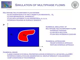
Y. X. Simulation of multiphase flows. Multiphase/multicomponent fluid systems Fluid domain W split in two o more fluid regions W 1 , W 2 Fluids separated by interface G Fluid with different fluid properties r 1 , m 1 , r 2 , m 2 Interface provided by surface tension s.


Simulation of multiphase flows
E N D
Presentation Transcript
Y X Simulation of multiphase flows • Multiphase/multicomponent fluid systems • Fluid domain W split in two o more fluid regions W1, W2 • Fluids separated by interface G • Fluid with different fluid properties r1, m1, r2, m2 • Interface provided by surface tension s • Numerical simulation of Multiphase/multicomponent flows • Interface tracking • flow field solution • Flow field interface coupling G W1 W2 • Numerical approaches • Sharp interface approach • Diffuse interface approach • Numerical issues • Large change in physical properties across interface (i.e. air water r1/r21000) • Interface dissolution and generation (i.e. droplet breakup/coalescence ) • Jump conditions at the interface
Sharp interface approaches • Basic ideas • Interface is treated as sharp layer • Each fluid described by a set of Navier Stokes equations • Fluid properties change sharply across the interface • Boundary conditions at the interface (free boundary problem) • Independent interface tracking Navier Stokes fluid 1 Navier Stokes fluid 2 Stress and velocity boundary condition s at the interface • Interface tracking • Lagrangian tracking: (sharp interface) • Level set (transport equation of diffuse level function) • Front tracking (sharp interface) • Volume of fluid (transport equation of diffuse fraction function)
Sharp interface approaches • Drawbacks of flow field solution: • Application of a set of boundary conditions at the interface • Sharp variations of fluid properties at the interface, infinite gradients • Particular solution techniques should be developed (i.e. ghost fluid methods, …) • Smearing of fluid properties should be introduced (i.e. Immersed boundary method) • Drawbacks of Interface tracking • Level set, Volume of fluid: interface degradation and mass leakage (non conservative methods) • Level set, Volume of fluid: Interface re-initialization techniques required (remove interface degradation) • Sharp approaches cannot deal interface creation and dissolution Level set interface degradation Errors in curvature computation • Jump conditions are not correctly computed • Re-initialization introduce errors • mass leakage still persist
Y Y X X Diffuse Interface Approach • Interface is a finite thickness transition layer • Localized and controlled fluid mixing (even for immiscible fluids) • fluid properties change smoothly from between the fluids r r r2 r2 r1 r1
Y X Phase Field Modelling • Definition of a scalar order parameter • Two fluid system represented as a mixture • The order parameter represents the local mixture concentration • f = fM identifies the actual sharp interface f Bulk fluid 1 f=f+ Bulk fluid 2 f= fm Interfacial layer Interface position f= f- Fluid properties proportional the Order parameter • State of the system represented by a scalar field • Continuous over the domain • Smooth variations across the interfaces • Order parameter function of the position
The Cahn Hilliard Equation • Time evolution of the order parameter gives the evolution of the system • From the PFM, the system is modeled as a mixture of two fluids • The order parameter represents the fluid concentration • Evolution of the concentration given by convective diffusion equation • Mass diffusion flux to be determined • derivation from evolution of binary mixtures free energy • Thermodynamically consistent • First derivation: Cahn & Hilliard (1958, 1959) • Cahn Hilliard Equation • Cahn Hilliard equation o generalized mass diffusion equation • Evolution of an immiscible & partially-miscible multiphase fluid system • Interface evolution controlled by a chemical potential
The free energy functional • Thermodynamic chemical potential, by definition • Partial derivative of free energy functional with respect to the mixture concentration • Free energy functional defines the behavior of the system under analysis • Fluid repulsion in bulk fluid regions (bulk free energy) • Controlled fluid mixing in the interfacial regions (non-local free energy) • Bulk • Free energy • Non-Local • Free energy • Bulk Free energy or ideal free energy • Accounts for the fluid repulsion • Shows two stable (minima) solutions • Its simplest form is a double-well potential • Different formulations can represent more complex systems (tri-phase,…)
The free energy functional • Non-Local Free energy • Responsible for the interfacial fluid mixing • Depends on the order parameter gradients (non-local behavior) • Keeps in account the mixing energy stored into the interface • The chemical potential, using the double-well free energy • The cahn hilliard equation, using the double-well free energy
Interface Properties • The equilibrium profile of the order parameter across the interface • Free energy is at its minima • Chemical potential is null • Two uniform solutions (bulk fluid regions) • Non-uniform solution normal to the interface Uniform solution 1 Uniform solution 2 Mono-dimensional Non-uniform solution analytical non-uniform solution first derived by van der waals (1879) Capillary length 99% of the surface tension is stored in an interface thickness of 4.164 capillary lengths
Interface Properties • The free energy functional keeps in account the mixing energy • Mixing energy is stored into the interface • Capillary effects are catch by the model • Thermodynamic definition of surface tension holds at equilibrium • Coefficients a, b, k, of the free energy functional • Define the surface tension • Define Capillary width • Define equilibrium concentration • Cannot be independently defined • Mobility parameter M of the Cahn-Hillard equation • Controls the diffusivity in the interface • Gives the interface relaxation time • Surface tension definition holds at equilibrium • Interface should always be at equilibrium • Relaxation time lower than convective time • Mobility and interface thickens are not independent • scaling law between • Interface thickness and • mobility Magaletti (2013)
Flow field Coupling The Cahn-Hilliard equation accounts also for the convective effects • Convective effects • Flow field solution • Navier Stokes / continuity equations system • Coupling term dependent on the phase field • Phase field surface force • The Chan-Hilliard/Navier-Stokes equations system has first been derived by Hohenberg and Halperin (1977) (“model H”) • Phase field surface force yields to the surface tension stress tensor • Phase field dependent viscosity (viscosity ratio between fluids) • Density matched fluids • Density mismatches require the solution of compressible Navier Stokes
Dimensionless Equations Dimensionless Cahn-Hilliard equation and Chemical potential Dimensionless Navier-Stokes/Continuity Non-Dimensional groups Reynolds Number Cahn number: Dimensionless interface thickness Peclet number: Dimensionless interface relaxation time Weber number: Inertia vs. Surface tension Dimensionless mobility
Advantages • Overcoming of sharp interface models problems • Absence of boundary conditions on the interface • Interface creation and dissolution cached • Interfacial layer do not degrade (conservative) Errors in curvature computation • Surface tension effects applied by a smeared surface force. No interfacial boundary conditions Level-Set (interface tracking for sharp interface approaches) interface Degradation Diffuse Interface Model Conservative interface
Advantages • Reliability of the model • Thermodynamically consistent • Conservative interfacial layer • convergence to Sharp interface limit • Consistent interface tracking and flow field coupling • Flexibility, different phenomena can be analyzed • Near critical phenomena • Morphology evolution • Droplet breakup /coalescence • ….
Drawbacks • Diffuse interface approximation • non physical interface thickness for immiscible fluids (Real thickness O(10-6)m) • Interfacial layer resolution require at least three mesh points • High resolution simulations required • Cahn Hilliard Numerical solution • Involves high order operators (up to 4th order) • thin interfacial layers involve high gradients • robust numerical algorithms required 4th order operator ensures the Conservation of interfacial layer
Droplet under shear flow Typical two phase flows benchmark, analytical solution is known Newtonian fluids; matched densities; matched viscosities; constant mobility. Dimensionless groups Dimensionless Governing Equations boundary conditions • Pseudo-spectral DNS: Fourier modes (1D FFT) in the homogeneous directions (x and y), • Chebychev coefficients in the wall-normal direction (z) • Time integration: Adams-Bashforth (convective terms), Crank-Nicolson (viscous terms)
Droplet under shear flow Deformation analysis, comparison with taylor (1921) Droplet deforms as a prolate ellipsoid of major axis L and minor axis b q Z Taylor law, valid for small Deformations D < 0.3 B Major axis orientation converge to 45° Y L The actual Capillary number depends on droplet initial radius and shear rate (Taylor 1921) X Deformation Parameter
Droplet under shear flow Deformation analysis, comparison with taylor (1921) Re = 0.2 Ch = 0.05 Pe = 20 Grid 128x128x129 t = 10-5 q=45° • Matching with Taylor law • Correct orientation of the deformed droplet • Minor discrepancies due to finite Reynolds number and interface identification
Droplet deformation an breakup In turbulent flows Newtonian fluids; matched densities; matched viscosities; constant mobility. Dimensionless groups Governing Equations • Time-dependent 3D turbulent flow at Ret=100 • Wide range of surface tension We=0.1 10 • Pseudo-spectral DNS: Fourier modes (1D FFT) in the homogeneous directions (x and y), • Chebychev coefficients in the wall-normal direction (z) • Time integration: Adams-Bashforth (convective terms), Crank-Nicolson (viscous terms)
Droplet deformation an breakup In turbulent flows Interface described by three mesh-points Simulation parameters: Physical parameters: Water flow
Droplet deformation an breakup In turbulent flows Qualitative analysis of deformation and breakup process Qian et al. (2006) Risso and Fabre (1998)
Droplet deformation an breakup In turbulent flows Deformation and breakup Diameter based Weber number Deformation parameter – Normalized external surface Breakup • Linear behavior of deformation with Weber number (Risso 1998) • Qualitative agreement with experiments of Risso and Fabre (1998) • Qualitative agreement with numerical Lattice Boltzmann results of Qian et al. (2006) No Breakup
Droplet deformation an breakup In turbulent flows Deformation behaviour, local curvatures probability density functions Undeformed droplet curvature Increasing Surface tension • Increasing surface tension reduce local deformability • Increasing principal curvature reduce the secondary curvature, incompressible interface
Droplet deformation an breakup In turbulent flows Oil in Water = 0.038N/m Wed = 0.085 = 0.002N/m Wed = 1.7
Droplet deformation an breakup In turbulent flows Oil in Water = 0.038N/m Wed = 0.085 = 0.002N/m Wed = 1.7 = 0.004N/m Wed = 0.85
Droplet deformation an breakup In turbulent flows Velocity field interface interactions, Analysis framework • Probability density functions of the velocity fluctuations Pdf of Velocity fluctuations inside the droplet Pdf of Velocity fluctuations outside the droplet • Statistics across the interface Z Z Analysis along the interface normal direction Y Y n ZG X X
Droplet deformation an breakup In turbulent flows Deformation and breakup • Fluctuations reduced inside the droplet • Similar behavior between different We • Outside the droplet fluctuations pdf similar to single-phase channel flow [Dinavahi et al. Phys. Fluids 7 (1995)]
Droplet deformation an breakup In turbulent flows Volume averaged turbulent kinetic energy Turbulent Kinetic Energy modulation observed for all surfece tensions. Different responses from external turbulent forcing Turbulent kinetic energy conserved in the wole channel
Droplet deformation an breakup In turbulent flows Volume Averaged Mean Total Kinetic Energy
Droplet deformation an breakup In turbulent flows n t2 t1 Z Y Oil in Water = 0.038N/m Wed = 0.085 X = 0.002N/m Wed = 1.7