Scalable Algorithms for Mining Large Databases
Scalable Algorithms for Mining Large Databases. Rajeev Rastogi and Kyuseok Shim Lucent Bell laboratories http://www.bell-labs.com/project/serendip. Overview. Introduction Association Rules Classification Clustering Similar Time Sequences Similar Images Outliers Future Research Issues


Scalable Algorithms for Mining Large Databases
E N D
Presentation Transcript
Scalable Algorithms for Mining Large Databases Rajeev Rastogi and Kyuseok Shim Lucent Bell laboratories http://www.bell-labs.com/project/serendip
Overview • Introduction • Association Rules • Classification • Clustering • Similar Time Sequences • Similar Images • Outliers • Future Research Issues • Summary
Background • Corporations have huge databases containing a wealth of information • Business databases potentially constitute a goldmine of valuable business information • Very little functionality in database systems to support data mining applications • Data mining: The efficient discovery of previously unknown patterns in large databases
Applications • Fraud Detection • Loan and Credit Approval • Market Basket Analysis • Customer Segmentation • Financial Applications • E-Commerce • Decision Support • Web Search
Data Mining Techniques • Association Rules • Sequential Patterns • Classification • Clustering • Similar Time Sequences • Similar Images • Outlier Discovery • Text/Web Mining
What are challenges? • Scaling up existing techniques • Association rules • Classifiers • Clustering • Outlier detection • Identifying applications for existing techniques • Developing new techniques for traditional as well as new application domains • Web • E-commerce
Examples of Discovered Patterns • Association rules • 98% of people who purchase diapers also buy beer • Classification • People with age less than 25 and salary > 40k drive sports cars • Similar time sequences • Stocks of companies A and B perform similarly • Outlier Detection • Residential customers for telecom company with businesses at home
Association Rules • Given: • A database of customer transactions • Each transaction is a set of items • Find all rules X => Y that correlate the presence of one set of items X with another set of items Y • Example: 98% of people who purchase diapers and baby food also buy beer. • Any number of items in the consequent/antecedent of a rule • Possible to specify constraints on rules (e.g., find only rules involving expensive imported products)
Association Rules • Sample Applications • Market basket analysis • Attached mailing in direct marketing • Fraud detection for medical insurance • Department store floor/shelf planning
Confidence and Support • A rule must have some minimum user-specified confidence 1 & 2 => 3 has 90% confidence if when a customer bought 1 and 2, in 90% of cases, the customer also bought 3. • A rule must have some minimum user-specified support 1 & 2 => 3 should hold in some minimum percentage of transactions to have business value
Example • Example: • For minimum support = 50%, minimum confidence = 50%, we have the following rules 1 => 3 with 50% support and 66% confidence 3 => 1 with 50% support and 100% confidence
Problem Decomposition 1. Find all sets of items that have minimum support • Use Apriori Algorithm • Most expensive phase • Lots of research 2. Use the frequent itemsets to generate the desired rules • Generation is straight forward
Problem Decomposition - Example For minimum support = 50% = 2 transactions and minimum confidence = 50% • For the rule 1 => 3: • Support = Support({1, 3}) = 50% • Confidence = Support({1,3})/Support({1}) = 66%
The Apriori Algorithm • Fk : Set of frequent itemsets of size k • Ck : Set of candidate itemsets of size k F1 = {large items} for ( k=1; Fk != 0; k++) do { Ck+1 = New candidates generated from Fk foreach transaction t in the database do Increment the count of all candidates in Ck+1 that are contained in t Fk+1 = Candidates in Ck+1 with minimum support } Answer = Uk Fk
Key Observation • Every subset of a frequent itemset is also frequent=> a candidate itemset in Ck+1 can be pruned if even one of its subsets is not contained in Fk
Apriori - Example Database D F1 C1 Scan D C2 C2 F2 Scan D
Efficient Methods for Mining Association Rules • Apriori algorithm [Agrawal, Srikant 94] • DHP (Aprori+Hashing) [Park, Chen, Yu 95] • A k-itemset is in Ck only if it is hashed into a bucket satisfying minimum support • [Savasere, Omiecinski, Navathe 95] • Any potential frequent itemset appears as a frequent itemset in at least one of the partitions
Efficient Methods for Mining Association Rules • Use random sampling [Toivonen 96] • Find all frequent itemsets using random sample • Negative border: infrequent itemsets whose subsets are all frequent • Scan database to count support for frequent itemsets and itemsets in negative border • If no itemset in negative border is frequent, no more passes over database needed • Otherwise, scan database to count support for candidate itemsets generated from negative border
Efficient Methods for Mining Association Rules • Dynamic Itemset Counting [Brin, Motwani, Ullman, Tsur 97] • During a pass, if itemset becomes frequent, then start counting support for all supersets of itemset (with frequent subsets) • FUP [Cheung, Han, Ng, Wang 96] • Incremental algorithm • A k-itemset is frequent in DB U db if it is frequent in both DB and db • For frequent itemsets in DB, merge counts for db • For frequent itemsets in db, examine DB to update their counts
Parallel and Distributed Algorithms • PDM [Park, Chen, Yu 95] • Use hashing technique to identify k-itemsets from local database • [Agrawal, Shafer 96] • Count distribution • FDM [Cheung, Han, Ng, Fy, Fu 96]
clothes footwear shirts outwear shoes hiking boots jackets pants Generalized Association Rules • Hierarchies over items (e.g. UPC codes) • Associations across hierarchies: • The rule clothes => footwear may hold even if clothes => shoes do not hold • [Srikant, Agrawal 95] • [Han, Fu 95]
Quantitative Association Rules • Quantitative attributes (e.g. age, income) • Categorical attributes (e.g. make of car) [Age: 30..39] and [Married: Yes] => [NumCars:2] • [Srikant, Agrawal 96] min support = 40% min confidence = 50%
Association Rules with Constraints • Constraints are specified to focus on only interesting portions of database • Example: find association rules where the prices of items are at most 200 dollars (max < 200) • Incorporating constraints can result in efficiency • Anti-monotonicity: • When an itemset violates the constraint, so does any of its supersets (e.g., min >, max <) • Apriori algorithm uses this property for pruning • Succinctness: • Every itemsetthat satisfies the constraint can be expressed as X1UX2U…. (e.g., min <)
Association Rules with Constraints • [Ng, Lakshmanan, Han, Pang 98] • Algorithms: Apriori+, Hybrid(m), CAP=> push anti-montone and succinct constraints into the counting phase to prune more candidates • Pushing constraints pays off compared to post-processing the result of Apriori algorithm
Temporal Association Rules • Can describe the rich temporal character in data • Example: • {diaper} -> {beer} (support = 5%, confidence = 87%) • Support of this rule may jump to 25% between 6 to 9 PM weekdays • Problem: How to find rules that follow interesting user-defined temporal patterns • Challenge is to design efficient algorithms that do much better than finding every rule in every time unit • [Ozden, Ramaswamy, Silberschatz 98] • [Ramaswamy, Mahajan, Silberschatz 98]
Optimized Rules • Given: a ruleandX => Y • Example: balance [l, u] => cardloan = yes. • Find values for land u such that support is greater than certain threshold and maximize a parameter • Optimized confidence rule: Given min support, maximize confidence • Optimized support rule: Given min confidence, maximize support • Optimized gain rule: Given min confidence, maximize gain
Optimized Rules • [Fukuda, Morimoto, Morishita, Tokuyama 96a] [Fukuda, Morimoto, Morishita, Tokuyama 96b] • Use convex hull techniques to reduce complexity • Allow one or two two numeric attributes with one instantiation each • [Rastogi, Shim 98], [Rastogi, Shim 99], [Brin, Rastogi, Shim99] • Generalize to have disjunctions • Generalize to have arbitrary number of attributes • Work for both numeric and categorical attributes • Branch and bound algorithm, Dynamic programming algorithm
Correlation Rules • Association rules do not capture correlations • Example: • Suppose 90% customers buy coffee, 25% buy tea and 20% buy both tea and coffee • {tea} => {coffee} has high support 0.2 and confidence 0.8 • {tea, coffee} are not correlated • expected support of customers buying both is • 0.9 * 0.25 = 0.225
Correlation Rules • [BMS97] generalizes association rules to correlations based on chi-squared statistics • Correlation property is upward closed • If {1, 2} is correlated, then all supersets of {1, 2} are correlated • Problem: • Find all minimal correlated item sets with desired support • Use Apriori algorithm for support pruning and upward closure property to prune non-minimal correlated itemsets
Bayesian Networks • Efficient and effective representation of a probability distribution • Directed acyclic graph • Nodes - random variables of interests • Edges - direct (causal) influence • Conditional probabilities for nodes given all possible combinations of their parents • Nodes are statistically independent of their non descendants given the state of their parents=> Can compute conditional probabilities of nodes given observed values of some nodes
Bayesian Network • Example1: Given the state of “smoker”, “emphysema” is independent of “lung cancer” • Example 2: Given the state of “smoker”, “emphysema” is not independent of “city “dweller” smoker city dweller emphysema lung cancer
Sequential Patterns • [Agrawal, Srikant 95], [Srikant, Agrawal 96] • Given: • A sequence of customer transactions • Each transaction is a set of items • Find all maximal sequential patterns supported by more than a user-specified percentage of customers • Example: 10% of customers who bought a PC did a memory upgrade in a subsequent transaction • 10% is the support of the pattern • Apriori style algorithm can be used to compute frequent sequences
Sequential Patterns with Constraints • SPIRIT [Garofalakis, Rastogi, Shim 99] • Given: • A database of sequences • A regular expression constraint R (e.g., 1(1|2)*3) • Problem: • Find all frequent sequences that also satisfy R • Constraint R is not anti-monotone=> pushing R deeper into computation increases pruning due to R, but reduces support pruning
Classification • Given: • Database of tuples, each assigned a class label • Develop a model/profile for each class • Example profile (good credit): • (25 <= age <= 40 and income > 40k) or (married = YES) • Sample applications: • Credit card approval (good, bad) • Bank locations (good, fair, poor) • Treatment effectiveness (good, fair, poor)
Decision Trees CreditAnalysis salary < 20000 yes no education in graduate accept yes no accept reject
Decision Trees • Pros • Fast execution time • Generated rules are easy to interpret by humans • Scale well for large data sets • Can handle high dimensional data • Cons • Cannot capture correlations among attributes • Consider only axis-parallel cuts
Decision Tree Algorithms • Classifiers from machine learning community: • ID3[Qui86] • C4.5[Qui93] • CART[BFO84] • Classifiers for large database: • SLIQ[MAR96], SPRINT[SAM96] • SONAR[FMMT96] • Rainforest[GRG98] • Pruning phase followed by building phase
Decision Tree Algorithms • Building phase • Recursively split nodes using best splitting attribute for node • Pruning phase • Smaller imperfect decision tree generally achieves better accuracy • Prune leaf nodes recursively to prevent over-fitting
SPRINT • [Shafer, Agrawal, Manish 96] • Building Phase • Initialize root node of tree • while a node N that can be split exists • for each attribute A, evaluate splits on A • use best split to split N • Use gini index to find best split • Separate attribute lists maintained in each node of tree • Attribute lists for numeric attributes sorted
Root education in graduate no yes SPRINT
Rainforest • [Gehrke, Ramakrishnan, Ganti 98] • Use AVC-set to compute best split: • AVC-set maintains count of tuples for distinct attribute value, class label pairs • Algorithm RF-Write • Scan tuples for a partition to construct AVC-set • Compute best split to generate k partitions • Scan tuples to partition them across k partitions • Algorithm RF-Read • Tuples in a partition are not written to disk • Scan database to produce tuples for a partition • Algorithm RF-Hybrid is a combination of the two
BOAT • [Gehrke, Ganti, Ramakrishnan, Loh 99] • Phase 1: • Constructb bootstrap decision trees using samples • For numeric splits, compute confidence intervals for split value • Perform single pass over database to determine exact split value • Phase 2: • Verify at each node that split is indeed the “best” • If not, rebuild subtree rooted at node
Pruning Using MDL Principle • View decision tree as a means for efficiently encoding classes of records in training set • MDL Principle: best tree is the one that can encode records using the fewest bits • Cost of encoding tree includes • 1 bit for encoding type of each node (e.g. leaf or internal) • Csplit : cost of encoding attribute and value for each split • n*E: cost of encoding the n records in each leaf (E is entropy)
Pruning Using MDL Principle • Problem: to compute the minimum cost subtree at root of built tree • Suppose minCN is the cost of encoding the minimum cost subtree rooted at N • Prune children of a node N if minCN = n*E+1 • Compute minCN as follows: • N is leaf: n*E+1 • N has children N1 and N2: min{n*E+1,Csplit+1+minCN1+minCN2} • Prune tree in a bottom-up fashion
Root education in graduate no yes 3.8 salary < 40k N MDL Pruning - Example no yes 1 1 N1 N2 • Cost of encoding records in N (n*E+1) = 3.8 • Csplit = 2.6 • minCN = min{3.8,2.6+1+1+1} = 3.8 • Since minCN = n*E+1, N1 and N2 are pruned
PUBLIC • [Rastogi, Shim 98] • Prune tree during (not after) building phase • Execute pruning algorithm (periodically) on partial tree • Problem: how to compute minCN for a “yet to be expanded” leaf N in a partial tree • Solution: compute lower bound on the subtree cost at N and use this as minCN when pruning • minCN is thus a “lower bound” on the cost of subtree rooted at N • Prune children of a node N if minCN= n*E+1 • Guaranteed to generate identical tree to that generated by SPRINT
5.8 N education in graduate no yes 1 N1 N2 1 PUBLIC(1) • Simple lower bound for a subtree: 1 • Cost of encoding records in N = n*E+1 = 5.8 • Csplit = 4 • minCN = min{5.8, 4+1+1+1} = 5.8 • Since minCN = n*E+1, N1 and N2 are pruned
PUBLIC(S) Theorem: The cost of any subtree with s splits and rooted at node N is at least 2*s+1+s*log a + • a is the number of attributes • k is the number of classes • ni (>= ni+1) is the number of records belonging to class i Lower bound on subtree cost at N is thus the minimum of: • n*E+1 (cost with zero split) • 2*s+1+s*log a + k å ni i=s+2 k å ni i=s+2
Bayesian Classifiers • Example: Naive Bayes • Assume attributes are independent given the class • Pr(C|X) = Pr(X|C)*Pr(C)/Pr(X) • Pr(X|C) = Pr(Xi|C) • Pr(X) = Pr(X|Cj)
C A2 An A1 Naive Bayesian Classifiers • Very simple • Requires only single scan of data • Conditional independence != attribute independence • Works well and gives probabilities