Download
1 / 71
720 likes | 916 Vues
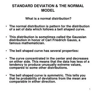
Chapter 6 The Standard Deviation and the Normal Model. 68-95-99.7 rule. Mean and Standard Deviation (numerical). Histogram (graphical). 68-95-99.7 rule. The 68-95-99.7 rule; applies only to mound-shaped data. 68-95-99.7 rule: 68% within 1 stan. dev. of the mean. 68%. 34%. 34%.

E N D
68-95-99.7 rule Mean and Standard Deviation (numerical) Histogram (graphical) 68-95-99.7 rule
68-95-99.7 rule: 68% within 1 stan. dev. of the mean 68% 34% 34% y-s y y+s
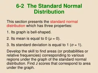
68-95-99.7 rule: 95% within 2 stan. dev. of the mean 95% 47.5% 47.5% y-2s y y+2s
Example: textbook costs 286 291 307 308 315 316 327 328 340 342 346 347 348 348 349 354 355 355 360 361 364 367 369 371 373 377 380 381 382 385 385 387 390 390 397 398 409 409 410 418 422 424 425 426 428 433 434 437 440 480
Example: textbook costs (cont.) 286 291 307 308 315 316 327 328 340 342 346 347 348 348 349 354 355 355 360 361 364 367 369 371 373 377 380 381 382 385 385 387 390 390 397 398 409 409 410 418 422 424 425 426 428 433 434 437 440 480
Example: textbook costs (cont.) 286 291 307 308 315 316 327 328 340 342 346 347 348 348 349 354 355 355 360 361 364 367 369 371 373 377 380 381 382 385 385 387 390 390 397 398 409 409 410 418 422 424 425 426 428 433 434 437 440 480
Example: textbook costs (cont.) 286 291 307 308 315 316 327 328 340 342 346 347 348 348 349 354 355 355 360 361 364 367 369 371 373 377 380 381 382 385 385 387 390 390 397 398 409 409 410 418 422 424 425 426 428 433 434 437 440 480
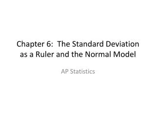
The best estimate of the standard deviation of the men’s weights displayed in this dotplot is • 10 • 15 • 20 • 40
Changing Units of Measurement Shifting data and rescaling data, and how shifting and rescaling data affect graphical and numerical summaries of data.
x* Shifts data by a a Changes scale 0 x Shifting and rescaling: linear transformations • Original data x1, x2, . . . xn • Linear transformation: x* = a + bx, (intercept a, slope b)
0 0 32 150 0 12 100 9/5 40 2.54 Linear Transformationsx* = a+ b x Examples: Changing • from feet (x) to inches (x*): x*=12x • from dollars (x) to cents (x*): x*=100x • from degrees celsius (x) to degrees fahrenheit (x*): x* = 32 + (9/5)x • from ACT (x) to SAT (x*): x*=150+40x • from inches (x) to centimeters (x*): x* = 2.54x
Shifting data only: b = 1x* = a + x • Adding the same value a to each value in the data set: • changes the mean, median, Q1 and Q3 by a • The standard deviation, IQR and variance are NOT CHANGED. • Everything shifts together. • Spread of the items does not change.
weights of 80 men age 19 to 24 of average height (5'8" to 5'10") x = 82.36 kg NIH recommends maximum healthy weight of 74 kg. To compare their weights to the recommended maximum, subtract 74 kg from each weight; x* = x – 74 (a=-74, b=1) x* = x – 74 = 8.36 kg Shifting data only: b = 1x* = a + x (cont.) • No change in shape • No change in spread • Shift by 74
Original x data: x1, x2, x3, . . ., xn Summary statistics: mean x median m 1st quartile Q1 3rd quartile Q3 stand dev s variance s2 IQR x* data: x* = a + bx x1*, x2*, x3*, . . ., xn* Summary statistics: new mean x* = a + bx new median m* = a+bm new 1st quart Q1*= a+bQ1 new 3rd quart Q3* = a+bQ3 new stand dev s* = b s new variance s*2 = b2 s2 new IQR* = b IQR Shifting and Rescaling data: x* = a + bx, b > 0
weights of 80 men age 19 to 24, of average height (5'8" to 5'10") x = 82.36 kg min=54.30 kg max=161.50 kg range=107.20 kg s = 18.35 kg Change from kilograms to pounds: x* = 2.2x (a = 0, b = 2.2) x* = 2.2(82.36)=181.19 pounds min* = 2.2(54.30)=119.46 pounds max* = 2.2(161.50)=355.3 pounds range*= 2.2(107.20)=235.84 pounds s* = 18.35 * 2.2 = 40.37 pounds Rescaling data: x* = a + bx, b > 0 (cont.)
4 student heights in inches (x data) 62, 64, 74, 72 x = 68 inches s = 5.89 inches Suppose we want centimeters instead: x* = 2.54x (a = 0, b = 2.54) 4 student heights in centimeters: 157.48 = 2.54(62) 162.56 = 2.54(64) 187.96 = 2.54(74) 182.88 = 2.54(72) x* = 172.72 centimeters s* = 14.9606 centimeters Note that x* = 2.54x = 2.54(68)=172.2 s* = 2.54s = 2.54(5.89)=14.9606 Example of x* = a + bx not necessary!UNC method Go directly to this. NCSU method
x data: Percent returns from 4 investments during 2003: 5%, 4%, 3%, 6% x = 4.5% s = 1.29% Inflation during 2003: 2% x* data: Inflation-adjusted returns. x* = x – 2% (a=-2, b=1) x* data: 3% = 5% - 2% 2% = 4% - 2% 1% = 3% - 2% 4% = 6% - 2% x* = 10%/4 = 2.5% s* = s = 1.29% x* = x – 2% = 4.5% –2% s* = s = 1.29% (note! that s* ≠ s – 2%) !! Example of x* = a + bx not necessary! Go directly to this
Example • Original data x: Jim Bob’s jumbo watermelons from his garden have the following weights (lbs): 23, 34, 38, 44, 48, 55, 55, 68, 72, 75 s = 17.12; Q1=37, Q3 =69; IQR = 69 – 37 = 32 • Melons over 50 lbs are priced differently; the amount each melon is over (or under) 50 lbs is: • x* = x 50 (x* = a + bx, a=-50, b=1) -27, -16, -12, -6, -2, 5, 5, 18, 22, 25 s* = 17.12; Q*1 = 37 - 50 =-13, Q*3 = 69 - 50 = 19 IQR* = 19 – (-13) = 32 NOTE: s* = s, IQR*= IQR
SUMMARY: Linear Transformations x* = a + bx • Linear transformations do not affect the shape of the distribution of the data -for example, if the original data is right-skewed, the transformed data is right-skewed
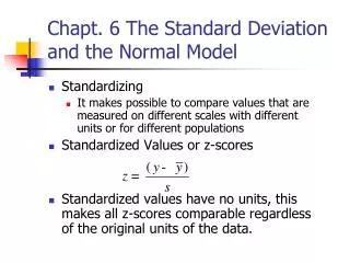
Z-scores: Standardized Data Values Measures the distance of a number from the mean in units of the standard deviation
Exam 1: y1 = 88, s1 = 6; exam 1 score: 91 Exam 2: y2 = 88, s2 = 10; exam 2 score: 92 Which score is better?
Comparing SAT and ACT Scores • SAT Math: Eleanor’s score 680 SAT mean =500 sd=100 • ACT Math: Gerald’s score 27 ACT mean=18 sd=6 • Eleanor’s z-score: z=(680-500)/100=1.8 • Gerald’s z-score: z=(27-18)/6=1.5 • Eleanor’s score is better.
Z-scores: a special linear transformation a + bx Example. At a community college, if a student takes x credit hours the tuition is x* = $250 + $35x. The credit hours taken by students in an Intro Stats class have mean x = 15.7 hrs and standard deviation s = 2.7 hrs. Question 1. A student’s tuition charge is $941.25. What is the z-score of this tuition? x* = $250+$35(15.7) = $799.50; s* = $35(2.7) = $94.50
Z-scores: a special linear transformation a + bx (cont.) Example. At a community college, if a student takes x credit hours the tuition is x* = $250 + $35x. The credit hours taken by students in an Intro Stats class have mean x = 15.7 hrs and standard deviation s = 2.7 hrs. Question 2. Roger is a student in the Intro Stats class who has a course load of x = 13 credit hours. The z-score is z = (13 – 15.7)/2.7 = -2.7/2.7 = -1. What is the z-score of Roger’s tuition? The linear transformation did not change the z-score! Roger’s tuition is x* = $250 + $35(13) = $705 Since x* = $250+$35(15.7) = $799.50; s* = $35(2.7) = $94.50 This is why z-scores are so useful!!
Nationally: Mean IQ=100 sd = 15 Average IQ by Browser Story was exposed as a hoax
NORMAL PROBABILITY MODELS The Most Important Model for Data in Statistics
X 0 3 6 9 12 8 µ = 3 and = 1 A family of bell-shaped curves that differ only in their means and standard deviations. µ = the mean = the standard deviation
Normal Probability Models • The mean, denoted ,can be any number • The standard deviation can be any nonnegative number • The total area under every normal model curve is 1 • There are infinitely many normal distributions
The effects of m and s How does the standard deviation affect the shape of f(x)? s= 2 s =3 s =4 How does the expected value affect the location of f(x)? m = 10 m = 11 m = 12
µ = 3 and = 1 X 0 3 6 9 12 µ = 6 and = 1 X 0 3 6 9 12
X 0 3 6 9 12 8 X 0 3 6 9 12 8 µ = 6 and = 2 µ = 6 and = 1
µ = 6 and = 2 X 0 3 6 9 12 area under the density curve between 6 and 8.
Standardizing • Suppose X~N( • Form a newrandom variable by subtracting the mean from X and dividing by the standard deviation : (X • This process is called standardizing the random variable X.
Standardizing (cont.) • (X is also a normal random variable; we will denote it by Z: Z = (X • has mean 0 and standard deviation 1:E(Z) = = 0; SD(Z) = = 1. • The probability distribution of Z is called the standard normal distribution.
Standardizing (cont.) • If X has mean and stand. dev. , standardizing a particular value of x tells how many standard deviations x is above or below the mean . • Exam 1: =80, =10; exam 1 score: 92 Exam 2: =80, =8; exam 2 score: 90 Which score is better?
X 0 3 6 9 12 .5 .5 8 (X-6)/2 Z -3 -2 -1 0 1 2 3 µ = 6 and = 2 µ = 0 and = 1
.5 .5 Z -3 -2 -1 0 1 2 3 Standard Normal Model Z = standard normal random variable = 0 and = 1 .5 .5
Important Properties of Z #1. The standard normal curve is symmetric around the mean 0 #2. The total area under the curve is 1; so (from #1) the area to the left of 0 is 1/2, and the area to the right of 0 is 1/2
Finding Normal Percentiles by Hand (cont.) • Table Z is the standard Normal table. We have to convert our data to z-scores before using the table. • The figure shows us how to find the area to the left when we have a z-score of 1.80:
.1587 Z Areas Under the Z Curve: Using the Table Proportion of area above the interval from 0 to 1 = .8413 - .5 = .3413 .50 .3413 0 1
Area between - and z0 Standard normal areas have been calculated and are provided in table Z. The tabulated area correspond to the area between Z= - and some z0 Z = z0
Example – begin with a normal model with mean 60 and stand dev 8 0.8944 0.8944 0.8944 0.8944 In this example z0 = 1.25