The Variance and Standard Deviation
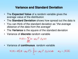
The Variance and Standard Deviation. The most important measure of variability is based on deviations of individual observations about the central value. For this purpose the mean usually serves as the center. MEASURES OF VARIABILITY. Variance Population variance Sample variance

The Variance and Standard Deviation
E N D
Presentation Transcript
The Variance and Standard Deviation The most important measure of variability is based on deviations of individual observations about the central value. For this purpose the mean usually serves as the center.
MEASURES OF VARIABILITY • Variance • Population variance • Sample variance • Standard Deviation • Population standard deviation • Sample standard deviation • Coefficient of Variation (CV) • Sample CV • Population CV
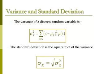
MEASURES OF VARIABILITYPOPULATION VARIANCE • The population variance is the mean squared deviation from the population mean: • Where 2stands for the population variance • is the population mean • N is the total number of values in the population • is the value of the i-th observation. • represents a summation
An example related to deviation about the central value • There are five SAT scores as below: 584, 613, 622, 693, 755. • The mean is (584+613+622+693+755)/5 = 653.4 • The deviation for each score can be computed by subtracting mean from each score: 755-653.4 = 101.6
An example related to deviation about the central value (cont..) 693-653.4 = 39.6 622-653.4 = -31.4 613.653.4 = -40.4 584-653.4 = -69.4 These deviations may be summarized by the collective measure that considers each deviation.
An example related to deviation about the central value (cont..) With the previous data, this procedure results in
Population Variance • In practice population variance cannot be computed directly because the entire population is not ordinarily observed. • An analogous measure of variability may be determined with sample data. • This referred to as sample variance
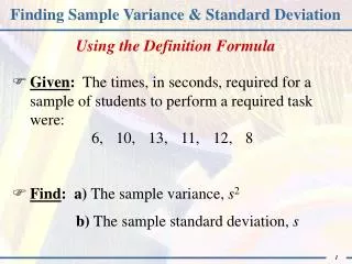
MEASURES OF VARIABILITYSAMPLE VARIANCE • The sample variance is defined as follows: • Where s2stands for the sample variance • is the sample mean • n is the total number of values in the sample • is the value of the i-th observation. • represents a summation
MEASURES OF VARIABILITYSAMPLE VARIANCE • Notice that the sample variance is defined as the sum of the squared deviations divided by n-1. • Sample variance is computed to estimate the population variance. • An unbiased estimate of the population variance may be obtained by defining the sample variance as the sum of the squared deviations divided by n-1 rather than by n. • Defining sample variance as the mean squared deviation from the sample mean tends to underestimate the population variance.
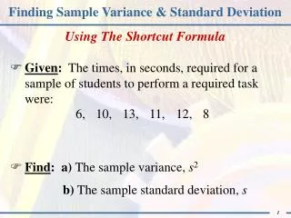
MEASURES OF VARIABILITYSAMPLE VARIANCE • A shortcut formula for the sample variance: • Where s2is the sample variance • n is the total number of values in the sample • is the value of the i-th observation. • represents a summation
MEASURES OF VARIABILITY POPULATION/SAMPLE STANDARD DEVIATION • The standard deviation is the positive square root of the variance: Population standard deviation: Sample standard deviation: • Compute the standard deviations of advertising and sales.
MEASURES OF VARIABILITY POPULATION/SAMPLE STANDARD DEVIATION • Compute the sample standard deviation of advertising data: 2.5, 1.3, 1.4, 1.0 and 2.0 • Compute the sample standard deviation of sales data: 264, 116, 165, 101 and 209
MEASURES OF VARIABILITY POPULATION/SAMPLE CV • The coefficient of variation is the standard deviation divided by the means Population coefficient of variation: Sample coefficient of variation:
MEASURES OF VARIABILITY POPULATION/SAMPLE CV • Compute the sample coefficient of variation of advertising data: 2.5, 1.3, 1.4, 1.0 and 2.0 • Compute the sample coefficient of variation of sales data: 264, 116, 165, 101 and 209
MEASURES OF ASSOCIATION • Scatter diagram plot provides a graphical description of positive/negative, linear/non-linear relationship • Some numerical description of the positive/negative, linear/non-linear relationship are obtained by: • Covariance • Population covariance • Sample covariance • Coefficient of correlation • Population coefficient of correlation • Sample coefficient of correlation
Sales Advertising Month (000 units) (000 $) 1 264 2.5 2 116 1.3 3 165 1.4 4 101 1.0 5 209 2.0 MEASURES OF ASSOCIATION: EXAMPLE • A sample of monthly advertising and sales data are collected and shown below: • How is the relationship between sales and advertising? Is the relationship linear/non-linear, positive/negative, etc.
POPULATION COVARIANCE • The population covariance is mean of products of deviations from the population mean: • Where COV(X,Y) is the population covariance • x,y are the population means of X and Y respectively • N is the total number of values in the population • are the values of the i-th observations of X and Y respectively. • represents a summation
SAMPLE COVARIANCE • The sample covariance is mean of products of deviations from the sample mean: • Where cov(X,Y) is the sample covariance • are the sample means of X and Y respectively • n is the total number of values in the population • are the values of the i-th observations of X and Y respectively. • represents a summation
POPULATION/SAMPLE COVARIANCE • If two variables increase/decrease together, covariance is a large positive number and the relationship is called positive. • If the relationship is such that when one variable increases, the other decreases and vice versa, then covariance is a large negative number and the relationship is called negative. • If two variables are unrelated, the covariance may be a small number. • How large is large? How small is small?
POPULATION/SAMPLE COVARIANCE • How large is large? How small is small? A drawback of covariance is that it is usually difficult to provide any guideline how large covariance shows a strong relationship and how small covariance shows no relationship. • Coefficient of correlation can overcome this drawback to a certain extent.
POPULATION COEFFICIENT OF CORRELATION • The population coefficient of correlation is the population covariance divided by the population standard deviations of X and Y: • Where is the population coefficient of correlation • COV(X,Y) is the population covariance • x,y are the population means of X and Y respectively
SAMPLE COEFFICIENT OF CORRELATION • The sample coefficient of correlation is the sample covariance divided by the sample standard deviations of X and Y: • Where r is the sample coefficient of correlation • cov(X,Y) is the sample covariance • sx,sy are the sample means of X and Y respectively
RELATIVE STANDINGBOX PLOTS • When the data set contains a small number of values, a box plot is used to graphically represent the data set. These plots involve five values: • the minimum value (S) • the lower quartile (Q1) • the median (Q2) • the upper quartile (Q3) • and the maximum value (L)
RELATIVE STANDING: BOX PLOTSEXAMPLE • Example: Construct a box plot with the following data which shows the assets of the 15 largest North American banks, rounded off to the nearest hundred million dollars: 111, 135, 217, 108, 51 , 98, 65, 85, 75, 75, 93, 64, 57, 56, 98
RELATIVE STANDING: BOX PLOTSINTERPRETATION • If the median is near the center of the box, the distribution is approximately symmetric. • If the median falls to the left of the center of the box, the distribution is positively skewed. • If the median falls to the right of the center of the box, the distribution is negatively skewed. • If the lines are about the same length, the distribution is approximately symmetric. • If the line segment to the right of the box is larger than the one to the left, the distribution is positively skewed. • If the line segment to the left of the box is larger than the one to the right, the distribution is positively skewed.
EXAMPLE • Salary and expenses for cultural activities, and sports related activities are collected from 100 households. Data of only 5 households shown below: How are the relationships (linear/non-linear, positive/negative) between (i) salary and culture, (ii) salary and sports, and (iii) sports and culture?