Spectral Line Observing
Spectral Line Observing. Ylva Pihlström, UNM. Introduction. Spectral line observers use many channels of width , over a total bandwidth . Why? Science driven: science depends on frequency (spectroscopy) Emission and absorption lines, and their Doppler shifts

Spectral Line Observing
E N D
Presentation Transcript
Spectral Line Observing Ylva Pihlström, UNM
Introduction • Spectral line observers use many channels of width , over a total bandwidth . Why? • Science driven: science depends on frequency (spectroscopy) • Emission and absorption lines, and their Doppler shifts • Slope across continuum bandwidth • Technical reasons: science does not depend on frequency (pseudo-continuum) Eleventh Synthesis Imaging Workshop, June 10-17, 2008
Spectroscopy • Need high spectral resolution to resolve spectral features • Example: SiO emission from a protostellar jet imaged with the VLA (Chandler & Richer 2001). • High resolutions over large bandwidths are useful for e.g., doppler shifts and line searches => many channels desirable! Eleventh Synthesis Imaging Workshop, June 10-17, 2008
Pseudo-continuum • Science does not depend on frequency, but using spectral line mode is favorable to correct for some instrumental responses: • Avoid limitations of bandwidth smearing • Avoid limitations of beam smearing • Avoid problems due to atmospheric changes as a function of frequency • Avoid problems due to signal transmission effects as a function of frequency • A spectral line mode also allows editing for unwanted, narrow-band interference. Eleventh Synthesis Imaging Workshop, June 10-17, 2008
2 Instrument response: beam smearing • θPB = l/D • Band covers l1 tol2 θPB changes by l1/l2 • More important at longer wavelengths: • VLA 20cm: 1.04 • VLA 2cm: 1.003 • EVLA 20cm: 2.0 • ALMA 1mm: 1.03 F. Owen Eleventh Synthesis Imaging Workshop, June 10-17, 2008
Instrument response: bandwidth smearing • Also called chromatic aberration • Fringe spacing = l/B • Band covers l1 tol2 • Fringe spacings change by l1/l2 • uv samples smeared radially • More important in larger configurations, and for lower frequencies • Huge effects for EVLA VLA-A 20cm: 1.04 Pseudo-continuum uses smaller ranges to be averaged later. Eleventh Synthesis Imaging Workshop, June 10-17, 2008
Instrument frequency response • Responses of antenna receiver, feed, IF transmission lines, electronics are a function of frequency. Tsys @ 7mm VLA • Phase slopes (delays) can be introduced by incorrect clocks or positions. VLBA Eleventh Synthesis Imaging Workshop, June 10-17, 2008
Atmosphere changes with frequency • Atmospheric transmission, phase (delay), and Faraday rotation are functions of frequency • Generally only important over very wide bandwidths, or near atmospheric lines • An issue for ALMA Chajnantor pvw = 1mm O2H2O • VLA pvw = 4mm • = depth of H2O if converted to liquid Eleventh Synthesis Imaging Workshop, June 10-17, 2008
EVLA: 1.2-2 GHz in one go VLA continuum bandwidth: 50 MHz RFI at the VLA, 1.2-1.8 GHz Radio Frequency Interference (RFI) • Avoid known RFI if possible, e.g. by constraining your bandwidth. • Possible in some cases but not always. RFI at MK, 1.6 GHz Eleventh Synthesis Imaging Workshop, June 10-17, 2008
Observations: data editing and calibration • Not fundamentally different from continuum observations, but a few additional items to consider: • Presence of RFI (data flagging) • Bandpass calibration • Doppler corrections • Correlator setup • Larger data sets Eleventh Synthesis Imaging Workshop, June 10-17, 2008
Editing spectral line data • Start with identifying problems affecting all channels, by using a frequency averaged 'Channel 0' data set. • Has better SNR. • Copy flag table to the line data. • Continue with checking the line data for narrow-band RFI that may not show up in averaged data. • Channel by channel impractical, instead identify features by using cross-power spectra (POSSM). • Is it limited in time? Limited to specific telescope (VLBI) or baseline length (VLA)? • Flag based on the feature using SPFLG, EDITR, TVFLG, WIPER. Eleventh Synthesis Imaging Workshop, June 10-17, 2008
Example POSSM scalar averaged spectra VLA • Note: avoid excessive frequency dependent editing, since this introduces changes in the u,v - coverage across the band. Eleventh Synthesis Imaging Workshop, June 10-17, 2008
Spectral response • For spectroscopy in an XF correlator (VLA, EVLA) additional lags are introduced and the correlation function is measured for a large number of lags. • The FFT gives the spectrum. • However, we don't have infinitely large correlators and infinite amount of time, so we don't measure an infinite number of Fourier components. • A finite number or lags means a truncated lag spectrum, which corresponds to multiplying the true spectrum by a box function. • The spectral response is the FT of the box, which for an XF correlator is a sinc(x) function with nulls spaced by the channel separation: 22% sidelobes! Eleventh Synthesis Imaging Workshop, June 10-17, 2008
Spectral response: Gibb's ringing "Ideal" spectrum Measured spectrum • Thus, this produces a "ringing" in frequency called the Gibbs phenomenon. • Occurs at sharp transitions: • Narrow banded spectral lines (masers, RFI) • Band edges • Baseband (zero frequency) Amp Amp Frequency Frequency Eleventh Synthesis Imaging Workshop, June 10-17, 2008
Gibb's ringing: remedies • Increase the number of lags, or channels. • Oscillations reduce to ~2% at channel 20, so discard affected channels. • Works for band-edges, but not for spectral features. • Smooth the data in frequency (i.e., taper the lag spectrum) • Usually Hanning smoothing is applied, reducing sidelobes to <3%. Eleventh Synthesis Imaging Workshop, June 10-17, 2008
Bandpass calibration • We need the total response of the instrument to determine the true visibilities from the observed: Vi j(t,)obs = Vi j(t,)Gi j(t) • The bandpass shape is a function of frequency, and is mostly due to electronics of individual antennas. • Usually varies slowly with time, so we can break the complex gain Gij(t) into a fast varying frequency independent part, G'ij(t,), and a slowly varying frequency dependent part Bij(t,): Vi j(t,)obs = Vi j(t,)G'i j(t)Bi j(t,) • G'i j(t) is calibrated as for continuum, and the process of determining Bi j(t,) is the bandpass calibration. Eleventh Synthesis Imaging Workshop, June 10-17, 2008
Why bandpass calibration is important • Important to be able to detect and analyze spectral features: • Frequency dependent amplitude errors limit the ability of detecting weak emission and absorption lines. • Frequency dependent phase errors can lead to spatial offsets between spectral features, imitating doppler motions. • Frequency dependent amplitude errors can imitate changes in line structures. • For pseudo-continuum, the dynamic range of final image is limited by the bandpass quality. Eleventh Synthesis Imaging Workshop, June 10-17, 2008
Example ideal and real bandpass Ideal Real Phase Phase • In the bandpass calibration we want to correct for the offset of the real bandpass from the ideal one (amp=1, phase=0). • The bandpass is the relative gain of an antenna/baseline as a function of frequency. Amp Amp Eleventh Synthesis Imaging Workshop, June 10-17, 2008
How BP calibration is performed • To compute the bandpass correction, a strong continuum calibrator is observed at least once. • The most commonly used method is analogous to channel by channel self-calibration (AIPS task BPASS) • The calibrator data is divided by a source model or continuum, which removes atmospheric and source structure effects. • Most frequency dependence is antenna based, and the antenna-based gains are solved for as free parameters. • This requires a high SNR, so what is a good choice of a BP calibrator? Eleventh Synthesis Imaging Workshop, June 10-17, 2008
How to select a BP calibrator • Select a continuum source with: • High SNR in each channel • Intrinsically flat spectrum • No spectral lines • Not required to be a point source, but helpful since the SNR will be the same in the BP solution for all baselines. Too noisy Spectral feature Spectra of three potential calibrators. Only the bottom one is ok. Strong, no lines: OK Eleventh Synthesis Imaging Workshop, June 10-17, 2008
How long to observe a BP calibrator • Applying the BP calibration means that every complex visibility spectrum will be divided by a complex bandpass, so noise from the bandpass will degrade all data. • Need to spend enough time on the BP calibrator so that SNRBPcal > SNRtarget. A good rule of thumb is to use SNRBPcal > 3SNRtarget which then results in an integration time: tBPcal = 3(Starget /SBPcal)2 ttarget Eleventh Synthesis Imaging Workshop, June 10-17, 2008
Assessing quality of BP calibration Amp Amp • Examples of good-quality bandpass solutions for 2 antennas. • Solutions should look comparable for all antennas. • Mean amplitude ~1 across useable portion of the band. • No sharp variations in amplitude and phase; variations are not dominated by noise. • Phase slope across the band indicates residual delay error. L. Matthews Eleventh Synthesis Imaging Workshop, June 10-17, 2008
Bad quality bandpass solutions four 4 antennas • Amplitude has different normalization for different antennas • Noise levels are high, and are different for different antennas L. Matthews Eleventh Synthesis Imaging Workshop, June 10-17, 2008
Bandpass quality: apply to a continuum source • Before accepting the BP solutions, apply to a continuum source and use cross-correlation spectrum to check: • That phases are flat • That amplitudes are constant • That the noise is not increased by applying the BP Before bandpass calibration After bandpass calibration Eleventh Synthesis Imaging Workshop, June 10-17, 2008
Spectral line bandpass: get it right! • G'ij(t) and Bij(,t) are separable, and multiplicative errors in G'ij(t) (including phase and gain calibration errors) can be reduced by subtracting structure in line-free channels. Residual errors will scale with the peak remaining flux. • This is not true for Bij(,t) - any errors in the bandpass calibration will always be in your data. Residual errors will scale as continuum fluxes in your observed field. Eleventh Synthesis Imaging Workshop, June 10-17, 2008
Doppler tracking • Observing from the surface of the Earth, our velocity with respect to astronomical sources is not constant in time or direction. • Doppler tracking can be applied in real time to track a spectral line in a given reference frame, and for a given velocity definition: Vradio/c = (nrest-nobs)/nrest Vopt/c = (nrest-nobs)/nobs Eleventh Synthesis Imaging Workshop, June 10-17, 2008
Rest frames Start with the topocentric frame, the successively transform to other frames. Transformations standardized by IAU. Eleventh Synthesis Imaging Workshop, June 10-17, 2008
Doppler tracking • However, the bandpass shape is really a function of frequency, not velocity! • Applying doppler tracking will introduce a time-dependent and position dependent frequency shift. • If you doppler track your BP calibrator to the same velocity as your source, it will be observed at a different sky frequency! • In this case, apply corrections during post-processing instead. • Given that wider bandwidths are now being used (EVLA, SMA, ALMA) online doppler tracking is unlikely to be used in the future (tracking only correct for a single frequency). Eleventh Synthesis Imaging Workshop, June 10-17, 2008
Continuum subtraction • Spectral line data often contains continuum emission, either from the target or from nearby sources in the field of view. • This emission complicates the detection and analysis of line data Spectral line cube with two continuum sources (structure independent of frequency) and one spectral line source. Roelfsma 1989 Eleventh Synthesis Imaging Workshop, June 10-17, 2008
Continuum subtraction: basic concept • Use channels with no line features to model the continuum • Subtract this continuum model from all channels Eleventh Synthesis Imaging Workshop, June 10-17, 2008
Why do continuum subtraction? • Spectral lines easier to see, especially weak ones. • Easier to compare the line emission between channels. • Deconvolution is non-linear: can give different results for different channels since u,v - coverage and noise differs (results usually better if line is deconvolved separately). • If continuum sources exists far from the phase center, we don't need to deconvolve a large field of view to properly account for their sidelobes. To remove the continuum, different methods are available: visibility based, image based, or a combination thereof. Eleventh Synthesis Imaging Workshop, June 10-17, 2008
Visibility based continuum subtraction (UVLIN) • A low order polynomial is fit to a group of line free channels in each visibility spectrum, the polynomial is then subtracted from whole spectrum. • Advantages: • Fast, easy, robust • Corrects for spectral index slopes across spectrum • Can do flagging automatically (based on residuals on baselines) • Can produce a continuum data set • Restrictions: • Channels used in fitting must be line free (a visibility contains emission from all spatial scales) • Only works well over small field of view << s / tot Eleventh Synthesis Imaging Workshop, June 10-17, 2008
UVLIN restriction: small field of view • A consequence of the visibility of a source being a sinusoidal function • For a source at distance l from phase center observed on baseline b: V = cos (2l/c) + i sin(2l/c) This is linear only over a small range of and for small b and l. Eleventh Synthesis Imaging Workshop, June 10-17, 2008
Image based continuum subtraction (IMLIN) • Fit and subtract a low order polynomial fit to the line free part of the spectrum measured at each spatial pixel in cube. • Advantages: • Fast, easy, robust to spectral index variations • Better at removing point sources far away from phase center (Cornwell, Uson and Haddad 1992). • Can be used with few line free channels. • Restrictions: • Can't flag data since it works in the image plane. • Line and continuum must be simultaneously deconvolved. Eleventh Synthesis Imaging Workshop, June 10-17, 2008
Visualizing spectral line data • After mapping all channels in the data set, we have a spectral line data cube. • The cube is 3-dimensional (RA, Dec, Velocity). To visualize the information we usually make 1-D or 2-D projections: • Line profiles (1-D slices along velocity axis) • Channel maps (2-D slices along velocity axis) • Position-velocity plots (slices along spatial dimension) • Moment maps (integration along the velocity axis) Eleventh Synthesis Imaging Workshop, June 10-17, 2008
Example: line profiles 3 3 4 • Line profiles shows changes in line shape, width and depth. • Right: EVN+MERLIN 1667 MHz OH maser emission and absorption spectra in IIIZw35. 10 1 5 11 2 6 12 7 4 13 8 9 10 5 1 11 6 2 12 7 13 8 9 Eleventh Synthesis Imaging Workshop, June 10-17, 2008
Example: channel maps • Channel maps show how the spatial distribution of the line feature changes with frequency/velocity. • Right: Contours continuum emission, grey scale 1667 MHz OH line emission in IIIZw35. Eleventh Synthesis Imaging Workshop, June 10-17, 2008
Example 2-D model: rotating disk +Vcir sin i cos +Vcir sin i -Vcir sin i -Vcir sin i cos Eleventh Synthesis Imaging Workshop, June 10-17, 2008
Velocity Right Ascension Declination Example: position-velocity plots • PV-diagrams shows, for example, the line emission velocity as a function of radius. Here along a line through the dynamical center of the galaxy Velocity profile Distance along slice • Greyscale & contours convey intensity of the emission. L. Matthews Eleventh Synthesis Imaging Workshop, June 10-17, 2008
Moment analysis • You might want to derive parameters such as integrated line intensity, centroid velocity of components and line widths - all as functions of positions. Estimate using the moments of the line profile: Total intensity (Moment 0) Intensity-weighted velocity (Moment 1) Intensity-weighted velocity dispersion (Moment 2) Eleventh Synthesis Imaging Workshop, June 10-17, 2008
Moment analysis Eleventh Synthesis Imaging Workshop, June 10-17, 2008
Moment maps Moment 0 Moment 1 Moment 2 (Total Intensity) (Velocity Field) (Velocity Dispersion) Eleventh Synthesis Imaging Workshop, June 10-17, 2008
Moment maps: caution! • Moments sensitive to noise so clipping is required • Higher order moments depend on lower ones so progressively noisier. • Hard to interpret correctly: • Both emission and absorption may be present, emission may be double peaked. • Biased towards regions of high intensity. • Complicated error estimates: number or channels with real emission used in moment computation will greatly change across the image. • Use as guide for investigating features, or to compare with other . • Alternatives…? • Gaussian fitting for simple line profiles. • Maxmaps shows emission distribution. Eleventh Synthesis Imaging Workshop, June 10-17, 2008
Velocity Right Ascension Declination Visualizing spectral line data: 3-D rendering L. Matthews Display produced using the 'xray' program in the karma software package (http://www.atnf.csiro.au/computing/software/karma/) Eleventh Synthesis Imaging Workshop, June 10-17, 2008