Spectral Line Imaging in Radio Astronomy: Understanding Basic Concepts and Techniques
260 likes | 329 Vues
Learn about spectral lines, photon-matter interactions, observation parameters, kinematics, and velocity reference frames in radio astronomy imaging. Explore calibration methods, continuum subtraction, data cubes, and moment maps for analyzing spectral data.

Spectral Line Imaging in Radio Astronomy: Understanding Basic Concepts and Techniques
E N D
Presentation Transcript
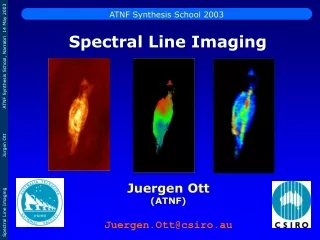
ATNF Synthesis School 2003 Spectral Line Imaging Juergen Ott (ATNF) Juergen.Ott@csiro.au
Topics • Introduction to Spectral Lines • Velocity Reference Frames • Bandpass Calibration • Continuum Subtraction • Gibbs Phenomenon & Hanning Smoothing • Data Cubes & Moment Maps Literature: Synthesis Imaging in Radio Astronomy II, Chapters 11 & 12 Synthesis Imaging in Radio Astronomy, Chapter 17
Introduction to Spectral Lines What is a spectral line ? Origin: Light dispersion (prisma, slit) sharp intensity maxima on screen “extent in frequency much less than central frequency of feature” S (n, n0, A,Dn,t) atomic/molecular origin
Introduction to Spectral Lines Basic photon–matter interactions to produce spectral lines: Absorption (e.g., towards quasars) Spontaneous emission (e.g., HI, molecular lines, cascading recombination lines) Induced emission (Maser/Laser) Continuum: free-free, free-bound recombination (e.g., synchrotron emission, thermal bremsstrahlung) E hn
HI 21cm - - + + Introduction to Spectral Lines • Energy levels can be: • Atoms: electron orbits, • hyperfine states • (UV, optical, IR, radio) • Nuclei: excitations (shell model), g radiation • Solid states: bands (IR, opt), lattice modes (phonons) • Molecules: (electronic+) rotation, vibration, bending • (mm, submm, IR) CO (carbon monoxide) NH3 (ammonia)
Introduction to Spectral Lines • What can we learn from spectral lines? • Observables: frequency, shape (width), amplitude, (time) • Parameters of the Gas • (density, temperature, pressure, column density, …) • Parameters of the Environment • (radiation field, maser conditions, chemistry, magnetic field) • Kinematics • (expansion/contraction, infall/outflow, rotation curves, • galaxy clusters, turbulence, virialization theorem) • Distance (Hubble Law v=H r)
l – l0 l – l0 n0 – n vopt = c = c z = c vradio = c l0 l n0 vopt = vradio Velocity Reference Frames Relativistic Doppler Effect: n02 – n2 vradial = n02 + n2 approximations for vradial << c
Correlator Configurations • Correlator Configurations: • Bandwidth • Channel Separation (# Channels) • # Blocks (simultaneous observations of different frequencies) • # polarization products Cold molecular gas: linewidth ~ few km s-1 Rotation curves: Amplitude ~200 km s-1
FT x R(t) I(n) * Gibbs Phenomenon, Hanning Smoothing BUT… Ideal: Lag (cross-correlation) spectrum R(t) measured from - to But: Digital cross-correlation spectrometer Truncation of time lag spectrum R(t) Gibbs phenomenon or Gibbs ringing sinc (x) = sin(x) / x Nulls spaced by channel separation I(n) I’(n)
…etc 0.25 0.25 0.25 0.25 0.5 0.5 Gibbs Phenomenon, Hanning Smoothing Solution • Observe with more channels than necessary • Tapering sharp end of lag spectrum R() • Hanning smoothing: f()=0.5+0.5 cos (/T) • In frequency space: multiply channels with 0.25, 0.5, 0.25 half velocity resolution w/o Hanning w/ Hanning
~ ~ ~ Vij (n,t) = Gij (n,t) Vij (n,t) complex measured visibility Gain calibrated visibility Bij (n,t) bi (n,t) bj* (n,t) Bandpass Calibration Calibration: Bandpass baseline Bandpass antenna Gij (n,t) = G’ij (t) Bij (n,t) Measurement: Strong point source with flat (known) spectrum: Bandpass Calibrator, noise source @ source frequency & correlator setup, maybe several times Strong enough for high S/N per individual channel! Solve from N(N-1)/2 baselines for N antennas
Bandpass Calibration Perfect Bandpass Amplitude Frequency / Channel
Continuum Subtraction Data: continuum + spectral line emission (several sources with different sizes) Continuum subtraction uv plane image plane uvlin (MIRIAD tasks) contsub Visibilities Spectra Pixel (real & imaginary) • Additional flagging can be applied • Better continuum map • Allows shifting of reference center on string source, then back • no deconvolution which is non-linear
Continuum Subtraction • select line free channels • low order polynomial fit for each visibility (real & imaginary) • subtract fit from spectrum line only line + continuum Line free channels result of bandpass correction: flag it!
Data Cubes Data Cubes Declinationd Velocity v Channel Maps Right Ascensiona
Data Cubes Channel Maps Spectrum
Data Cubes Expanding Shell
Data Cubes position velocity
Data Cubes position – velocity cuts Major axis cut velocity position Minor axis cut Declination velocity velocity position Right ascension
mi := (x-a)i f(x) dx a := v f(v) dv - - Data Cubes – Moment Maps Moment maps Mathematical definition of central i-th moment (statistics): f(x): probability distribution a: center of mass of f(x)
M1 M2 M0 Data Cubes – Moment Maps Important Moments (as actually calculated, S over all spectral channels for each pixel): 0th moment: integrated intensity map [Jy km s-1] M0 = S I(v) Dv 1st moment: intensity weighted velocity map [km s-1] M1 = S I(v) v / S I(v) i=2, 2nd moment: 1s velocity dispersion [km s-1] M2 = S [I(v) (v-M1)2] / S I(v) Caution!!
Data Cubes – Moment Maps Moment 0 Moment 1 Moment 2
Conclusion Conclusion: Spectral line imaging is… powerful, versatile, fun!!!