Physical Oceanography and Modeling Capabilities
Physical Oceanography and Modeling Capabilities. Cisco Werner UNC-Chapel Hill cisco@unc.edu. Eel workshop Blacksburg, 23 March 2005. Eel Life Cycle (as understood by a physical ocean modeler).

Physical Oceanography and Modeling Capabilities
E N D
Presentation Transcript
Physical Oceanography and Modeling Capabilities Cisco Werner UNC-Chapel Hill cisco@unc.edu Eel workshop Blacksburg, 23 March 2005
Eel Life Cycle (as understood by a physical ocean modeler) • The eel begins and ends its life in the waters of the Sargasso Sea, an area north of the Bahamas. • The leptocephalus, a pelagic larvae of less than two inches in length, drifts with the ocean currents for 9 to 12 months before entering coastal waters. • When it reaches approximately 2.4 inches (6 cm) in length, the leptocephalus metamorphoses into a transparent, "glass" eel. • In autumn the glass eels migrate into estuaries along the Atlantic coast where they become pigmented. These eels are known as elvers. • Some elvers remain in the estuaries, but others migrate varying distances upstream, often for several hundred kilometers. http://www.chesapeakebay.net/american_eel.htm
Major ocean current systems Spawning site
In the mid-1980s (in Europe), the number of new glass eels entering rivers declined to 10% of former levels and recent figures show that this has now dropped to 1%. The crash happened over the whole European continent with no single, obvious cause. Suggestions for possible causes have included over-exploitation, inland habitat loss, climate and ocean current change, disease and pollution. http://www.ices.dk/marineworld/eel.asp
10 year trajectories Fixed depth (no vertical displacement) 10 year trajectories Passive trajectories (free vertical motion)
Eddy-driven sources and sinks of nutrients in the upper ocean:results of a 0.1° resolution model of the North Atlantic McGillicuddy, D.J., Anderson, L.A., Doney, S.C. and M.E. Maltrud National Science Foundation NCAR: Scientific Computing Division
New Production in the Open Ocean
An eddy-resolving nutrient transport model Euphotic Zone: NP=NP(I,NO3,T) Aphotic Zone: Relaxation to clim. NO3(σT)
Simulated Annual New Production OWSI NABE BATS EUMELI
Annual New ProductionTerm Balances New Prod Conv + Diff Vertical advection Horizontal advection Total Mean Eddy
New Production at BATS:Three Models, Three Different Nutrient Transport Pathways Observed Annual New Production = 0.5 mol N m-2 yr-1
Coarse (1.6º) Eddy-resolving (0.1º) Sea Surface Temperature log (New Production)
1 2 4 3 5 6 Nested Grids in the Northwest Atlantic using ROMS • 1) NENA • 2) NEOS • 3) CBLAST4) LATTE • 5) NY/NJ Bight • 6) Caribbean • 7) Not shown: • Delaware Bay • Narragansett Bay • Chesapeake Bay • North Atlantic Basin
Northeast North Atlantic (NENA) embedded within NATL 3-day average open boundary values from NATL7-component NPZD ecosystem Temperature Chlorophyll
Residual flow field under average wind conditions October January March Wind Direction
Arrival at slack before ebb Arrival at slack before flood
Long-term changes in the ecology (hydro-climate + biology) of the North Sea (Beaugrand, in press PO)
Long-term changes in the abundance of two key species in the North Sea Percentage of C. helgolandicus (Beaugrand)
Long-term changes in the abundance of two key species in the North Sea Calanus finmarchicus Calanus helgolandicus 12 12 1.6 1 11 11 1.4 0.9 10 10 0.8 1.2 9 9 0.7 8 8 1 0.6 7 7 months 0.8 0.5 6 6 0.4 5 0.6 5 0.3 4 4 0.4 0.2 3 3 0.2 2 0.1 2 1 1 60 65 70 75 80 85 90 95 60 65 70 75 80 85 90 95 Years (1958-1999) Years (1958-1999) (Beaugrand)
Relevant Programs • GODAE – Global Ocean Data Assimilation Experiment (NASA) • CLIVAR – Climate Variability • OOI – Ocean Observatories Initiative (NSF) • GOOS – Global Ocean Observing System • IOOS – Integrated Ocean Observing System (NOAA)
Will follow IOOS model of overlapping regional systems that together form a national system
SEA-COOS The Southeast Atlantic Coastal Ocean Observing System
NC 1 Site SC 2 Sites GA 2000 m 2 Sites 200 m Fisheries Management ObservationsC. Barans, SCDNR Fisheries Observation Network Ecosystem Based Fisheries Management • Cyclic movements • Interactions • Spawning times • Recruitment High Temporal Resolution: Microwave Transmission System • Near real-time data Autonomous Video Loggers • Regional coverage • Latitudinal/ depth
System example: “FishCam” • C. Barans, SC DNR • video clips from 6-camera system • hourly images • telemetry via SABSOON • microwave/T1 communications Images from current day: www.skio.peachnet.edu/research/sabsoon /fishwatch/ Searchable video archive: http://oceanica.cofc.edu/FishWatch/open.htm Included are a Searchable Data Base and an Educational Web Site