Download
1 / 16
160 likes | 273 Vues
Combining Information from Related Regressions. F. Dominici, G. Parmigiani, K. H. Reckhow and R. L. Wolpert, JABES 1997. Duke University Machine Learning Group Presented by Kai Ni Apr. 27, 2007. Outline. Introduction Model Results Conclusion. Motivation. The general problem

E N D
Combining Information from Related Regressions F. Dominici, G. Parmigiani, K. H. Reckhow and R. L. Wolpert, JABES 1997 Duke University Machine Learning Group Presented by Kai Ni Apr. 27, 2007
Outline • Introduction • Model • Results • Conclusion
Motivation • The general problem • Combining of the individual studies in order to learn about the whole – Meta-analysis. • Here the author considers how to combine several multivariate regression data sets, each recording overlapping, but possibly different, sets of variables. • Why meta-analysis • Initial study may identify the relationship between variables and motivate new interesting explanatory variables. • Different studies may have multiple endpoints (responses).
Common modeling problems • Combining several studies with a common response variable and overlapping, but different covariates. • Combining studies with the same covariates but different endpoints (responses), with the aid of further studies investigating the dependence between the endpoints. • Combining multivariate analysis with different sets of variables. • Y = w0 + w1X1 + w2X2 + w3X3
A Tutorial Example • We have several studies of lake quality: effects of phosphorus (X1) on the concentration of chlorophyII-a (Y). • First study – correct for the effect of nitrogen (X2); • Second study – correct for the effect of lake depth (X3); • Third study – correct for the effect of both covariates (X2,X3); • Our goal is to combine information from the three studies to find the regression coefficients w for X1.
A Tutorial Example (2) • From the first study we findFrom the first study we find • From the second study we find • From the third study we find • X1 affecting Y though the first two studies agreed in w=0. • We should expand the multivariate regression model to include the uncertain joint distribution of all the covariates X’s, rather than only the conditional distribution of Y given X’s. (Missing feature problems)
Model for Complete Data (2) • Put common prior on the group-specific mean and covariance matrices. Also consider the uncertainty on the prior distribution, we have the following model: • Interest is both in the study specific (stage II) parameters and in the population (stage III) parameters.
Missing Variables (Incomplete data) • Now consider the situation where some of the variables are missing. We rearrange the vector Z, so that it can be written as (W, U ). • Both W and U can include responses and explanatory variables. • To deal with the missing data, draw samples of unknowns using the posterior distribution
Sampling • The posterior distribution is not available in closed form, therefore MCMC (block Gibbs sampler) is used for inference.
Chlorophyll-Phosphorus relations in Lakes • Study cases for investigating the relation between chlorophyll-a, phosphorus, and nitrogen in lakes. • Chlorophyll-a is one of the most widely measured and predicted indicators of lake water quality. Higher chlorophyll-a – higher algal densities – poorer water quality. • Data from 12 north temperate lakes. TP = total phosphorus; TN = total nigrogen; C = chlorophyll-a.
Model for this meta-analysis • It is necessary to include in the analysis the effect of the nitrogen, even though some studies do not report nitrogen levels; • It is of interest to investigate both the geographical and temporal dependencies between the variables and to model those separately, as temporal variation is more strongly related to human intervention; • It can be important to provide a predictive distribution for the effect of phosphorus concentration reduction in a north temperate lakes not included in the sample.
Results • Using the Gibbs sampler to obtain a sample from the join posterior distribution of all unknown quantities. • Samples of the vectors Bs (regression coefficients in each of the twelve lakes) and the vector B* (overall regression coefficients) can be obtained from the sampled parameters.
Inference on regression coefficients. Log(TP) (left) is relative stable while log(TN/TP) (right) is variable across lakes.
Left: Prior and posterior distributions on B* -- Data is strong even on stage III. Right: Joint distribution of beta1* and beta2* -- indicating strong correlation
Conclusion • Consider the problem of combining information from several regression studies. • Use Bayesian hierarchical models for study-to-study as well as within-study variability. • Provide full conditional distributions for the implementation of a Gibbs sampler, useful for missing variables in study.