Download
1 / 37
400 likes | 545 Vues
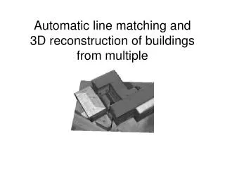
Automatic line matching and 3D reconstruction of buildings from multiple. Reference. Automatic line matching and 3D reconstruction of buildings from multiple views Baillard, C. , Schmid, C. , Zisserman, A. and Fitzgibbon, A.

E N D
Automatic line matching and 3D reconstruction of buildings from multiple
Reference • Automatic line matching and 3D reconstruction of buildings from multiple views • Baillard, C. , Schmid, C. , Zisserman, A. and Fitzgibbon, A. • ISPRS Conference on Automatic Extraction of GIS Objects from Digital Imagery, IAPRS Vol.32, Part 3-2W5 • Automatic Line matching across views. • C. Schmid and A. Zisserman. • CVPR 97(666-671). • http://www.robots.ox.ac.uk/~vgg • http://www.robots.ox.ac.uk/~impact
Contents 1. The IMPACT project 2. Line matching over multiple views 3. Producing piecewise planar models 4. Future works and extensions.
The IMPACT Project • The Image Processing for Automatic Cartographic Tools. • Bonn(Germany), Leuven (Belgium), Oxford (England), ENST(France), and Eurosense (Belgium). • The IMPACT Project Works with 4 to 6 images • Very high resolution data. (1200×1200) • Find matching lines in 3-D. • Generate surfaces as half-planes. • Generate new lines from intersections of these surfaces
, ,
Difficulty of Line matching • The deficiencies in extracting lines and their connectivity: • The end points are not reliable • Topological connections between line segments are often lost • No strong disambiguating geometric constraint available over 2 views: • Infinite lines there is no geometric constraint
Existing approaches to line matching • Match individual line segments • generally matched on their geometric attributes • orientation, length, extent of overlap • use a nearest line strategy • Match groups of line segments. • more geometric information • graph-matching • Topological connectedness. • left of, right of, cycles, collinear with etc,
Graph Matching • Stereo Correspondence Through Feature Grouping and Maximum Cliques.Horaud, R. and Skordas, T., 1989. IEEE TPAMI11(11), pp. 1168–1180. • Feature and Feature relation Correspondence graph • Stereo correspondence • Searching for set of mutually compatible node in graphs
Graph Matching Two images to be matched Two structural description to be matched.
Extracting Line segments • Canny edge detector • hysteresis threshold edges are linked to chain. • Jumping to one pixel gap. • Line segment fitting • Orthogonal regression • tight threshold curves are not linear approximated. • Before Line Matching • Fundamental matrix and Trifocal Tensor should be calculated from point correspondence
Image 2 Two view matching • F-guided matching (Line matching) two imaged line Image 1 The matching score : the average of the individual correlation scores for the points (pixels) of the line.
Three-view matching – – –
Three-view matching • If the geometric test is passed, the photometric test must also be passed. • 50% of the score threshold. • If the geometric test is not passed, the pair hypothesis can still be verified by the photometric test. • 50% more than the score threshold
Implementation detail • Minimum length : 15 pixels. • To robust to occlusion • Individual correlation value is only included if above a threshold. • correlation window : 15×15 ,The threshold 0.6 • “winner takes all” • a line belongs to several triples, only the triple with the best score is retained. • The lines are reconstructed in 3D by minimizing reprojection error • LM Method
, ,
Improving the quality of the matched lines • Merging • Before applying “winner takes all” • Growing • if a short line is matched to a longer line the end points may be extended
Extension to N-view matching • Using more views • reduces matching errors. • increases the accuracy of the estimated 3D line. • project the 3-view estimated line into subsequent images • Different method in this thesis line triple corresponding 3D line segment and reciprocally added to the matching set.
Three main stages • Computing reliable half-planes • similarity scores computed over all the views • The most important and novel stage • Line grouping and completion • grouping neighboring 3D lines belonging to the same half-plane • Plane delineation and verification
Computing half-planes • One parameter family of planes
Computing half-planes • The similarity score function : normalized cross-correlation : inversely proportional to the distance of the point x from the line L : recursive sub-division with a termination criterion of
Computing half-planes • The similarity score function projected 3D lines (white). Detected edges (black) : very low threshold on gradient. These edges provide the points of interest.
Example of similarity score functions The black curve corresponds to a valid plane, whereas the grey one is rejected. Whereas the grey one is rejected.
Computing half-planes Detected half-planes over the interval
Line grouping and completion • Collinear grouping • Two collinear lines which have attached coplanar half-planes are merged together.
Line grouping and completion • Coplanar line and half-plane grouping • line which is neighboring and coplanar with the current plane is associated with it
Line grouping and completion (a) (b) 3D line grouping.(a) Collinear grouping reduces the 9 planes prior to grouping to only 6. (b) Coplanar grouping and plane merging.
Line grouping and completion • Creating new lines by plane intersections Creation of new lines when two planes intersect.
Plane delineation and verification • Determining the closed border lines • using heuristic grouping rules : the area of the face, : the ratio of the length of input 3D lines to hypothesised lines in the delineation.
Plane delineation and verification (a) (b) Example of a reconstructed roof. (a) Delineation of the verified roofs projected onto the first image.(b) 3D view with texture mapping.
Model Reconstruction Result Model reconstruction results(a) 49 detected half-planes from 137 3D lines. (b) 3D model of the scene (12 roof planes). The vertical walls are produced by extruding the roof’s borders to the ground plane. (c) 3D model of the scene with texture mapping
Model Reconstruction Result Model reconstruction results on the large (1200×1200) images. (a) The 452 reconstructed 3D lines and the 267 detected half-planes. (b) and (c) Two views of the 3D model of the scene, with texture mapping (180 roof planes).
4. Future works and extensions • How might the quality be improved further? • Providing additional features for matching • Most significant • 3D grouping mechanism • The similarity score function • Require a firmer statistical foundation